Fotometria

Photometry

Lorenzo Franco- Roma

 11 marzo 2017

Estratto della relazione svolta al Convegno degli astrofili ricercatori

Fulvio Mete - Roma

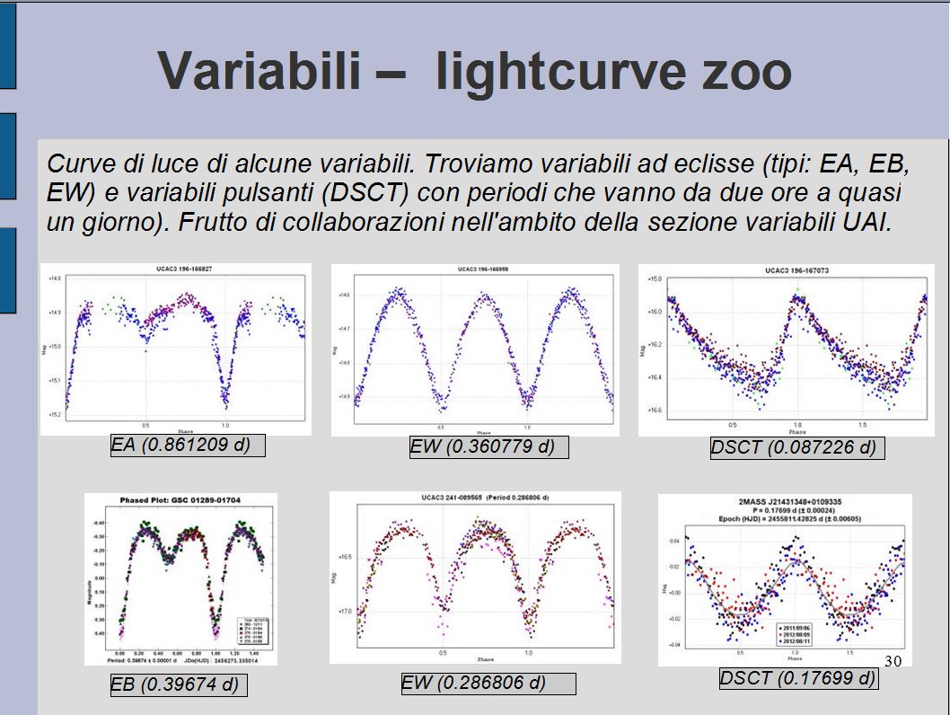
M27 e la variabile di  Goldilocks: scomparsa ed apparizione

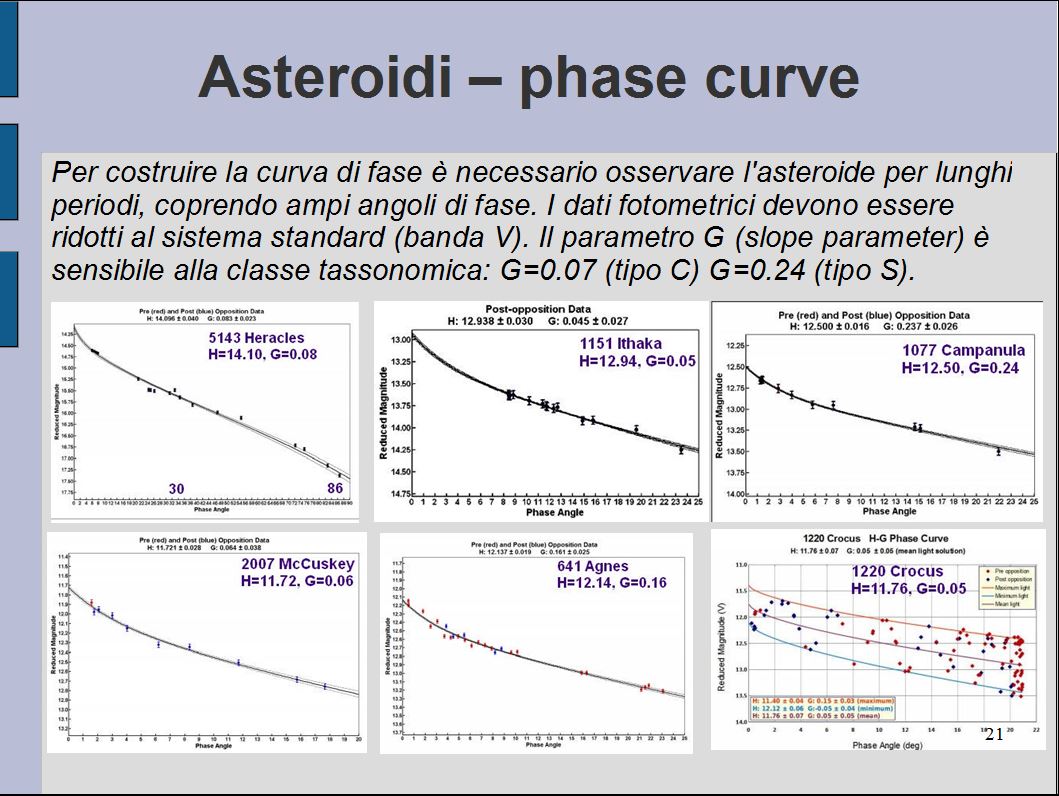
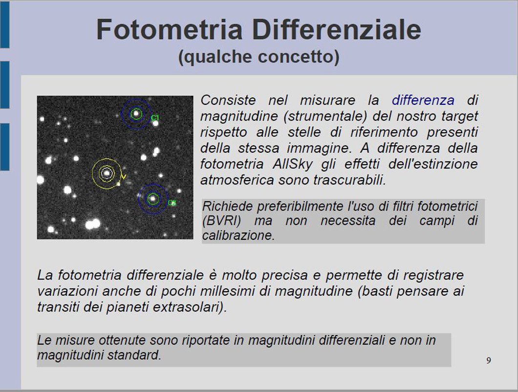
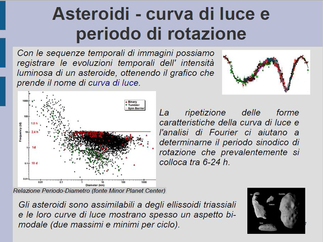
Su M27 c’è ormai ben poco da dire : è una delle nebulose planetarie più celebri, osservate e fotografate del cielo boreale.Fu scoperta da Messier nel 1764 e dista circa 1360 anni luce dalla terra, è di magnitudine apparente 7,4, ha un diametro apparente di circa 8 arcominuti  la sua forma ricorda quella di uno sferoide forma di manubrio (da cui il nome) ed è vista lungo la linea prospettica del piano equatoriale, l'età cinematica della nebulosa sarebbe di 9800 anni.La stella centrale, come molte nebulose planetarie, è una nana bianca.

Ben pochi tuttavia sono a conoscenza di due sue caratteristiche particolari:

1- Essa ospita (tra altre) una variabile a dir poco strana per due motivi, il primo che fu scoperta dall’astrofilo cecoslovacco Leos Ondra non attraverso il telescopio ed altro strumento ottico, ma …osservando due riviste  che riportavano in copertina un’immagine a colori di M27: il numero di Giugno 1990 di Astronomy, e quello di autunno dello stesso anno di Deep Sky.Ondra si accorse infatti che una stellina riportata sulla copertina della prima rivista non appariva in quella della seconda.Della stellina furono poi effettuati riscontri astrometrici e fotometrici, che confermarono essere una variabile di lungo periodo (214 gg) di tipo Mira (stelle rosse, massicce e pulsanti), alla quale fu dato il nome di “variabile di Goldilocks”. Ma non finisce qui: la stella è classificata anche come oggetto 2 Mass per la sua segnatura nell’IR vicino (J (1.25 μ ;  H, 1.65 μ  e K, 2.17 μ ).Esso è presente anche nella Survey WISE (3.4; 4.6; 12 e 22 μ)  ed è catalogato da Simbad come NSV 24959 alle coordinate : 19:59:29.72  + 22:45:13.0.

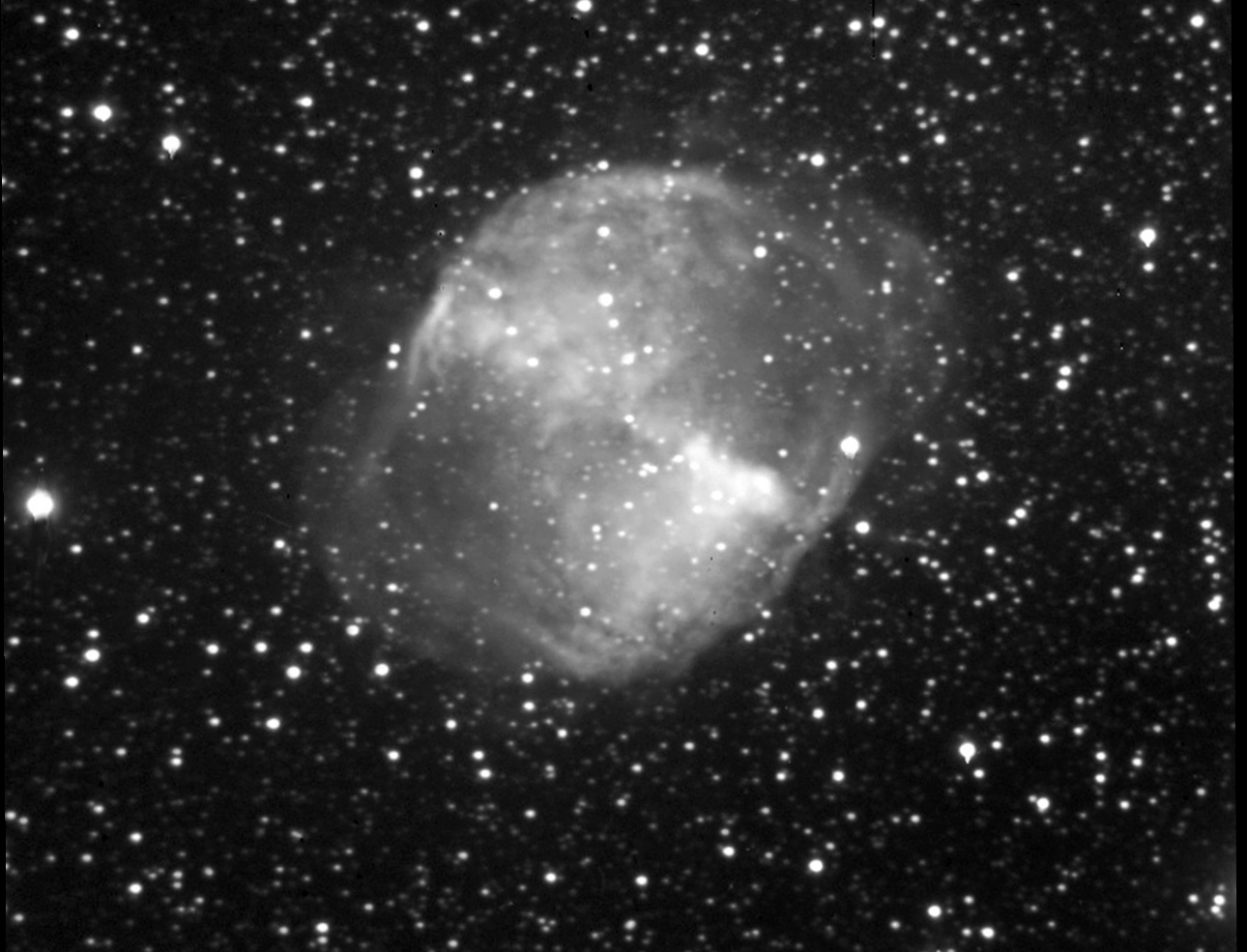
2 – Mentre nel visibile la nebulosa mostra i suoi splendidi colori, dal blu al rosso, come si può osservare nella prima immagine allegata, nell’IR vicino al di sotto del micron essa scompare letteralmente, grazie anche al potere di penetrazione dell’IR nell’inviluppo di gas e polveri.

 In un breve periodo di vacanza  dell lugnio 2019 ho quindi voluto sperimentare tali caratteristiche di M27:

1- effettuando riprese CCD dell’intera nebulosa:

     a) in LRGB

     b) con filtro UHC

     c)  con filtro Neodymium (Anti IL)

     d) senza filtri

     e) con filtro IR Pass > 742 nm

La strumentazione usata è stata un telescopio Schmidt Cassegrain Celestron 8 ridotto a f 6.3 ed una camera Sbig ST 10 usata in binning 1x1.

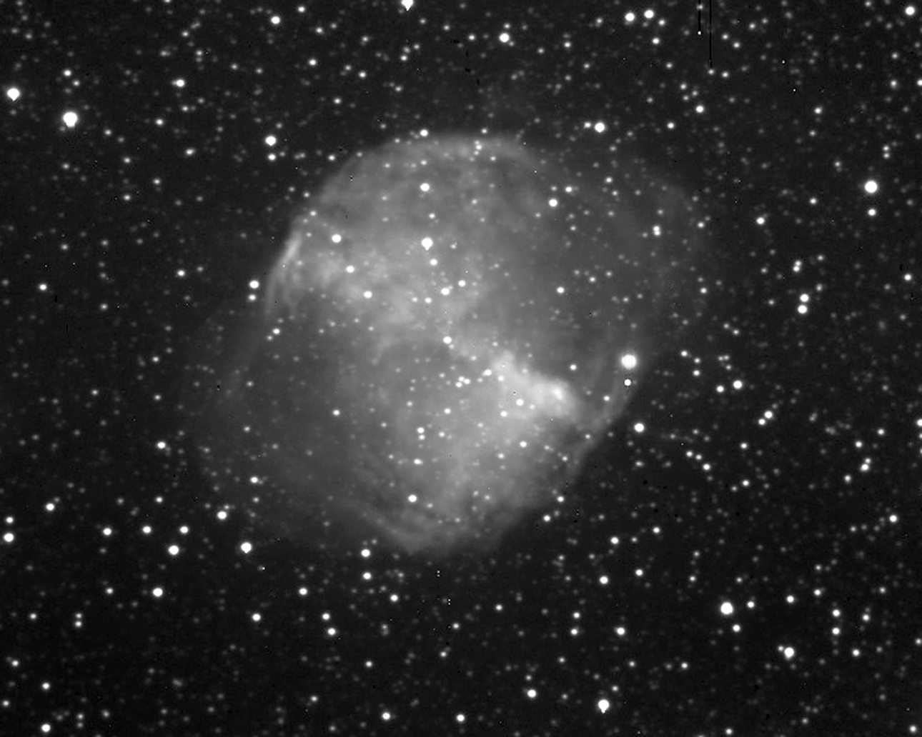
Nell’immagine n1 è mostrata l’usuale LRGB della nebulosa con evidenziata la variabile di Goldilocks; nella seconda quella col filtro Astronomik UHC , nella terza quella con un Baader Neodymium,nella quarta quella senza filtri, e nella quinta quella con un Astronomik IR Pass 742.Mentre le variazioni nell’apparenza della nebulosa coi vari filtri sono modeste , quella tra l’immagine Raw senza filtri e quella nell’IR vicino è drammatica, con la pratica scomparsa della nebulosa stessa.

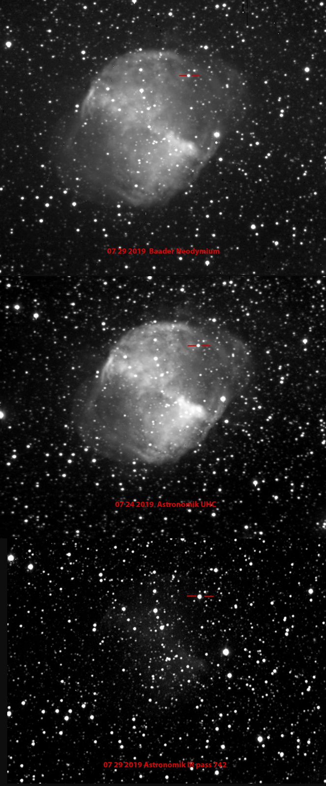
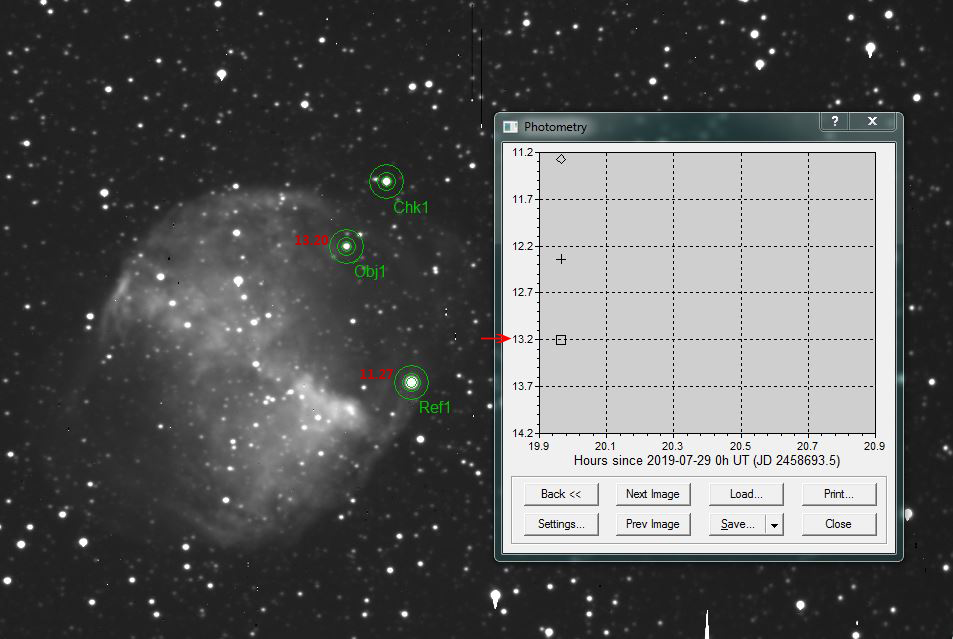
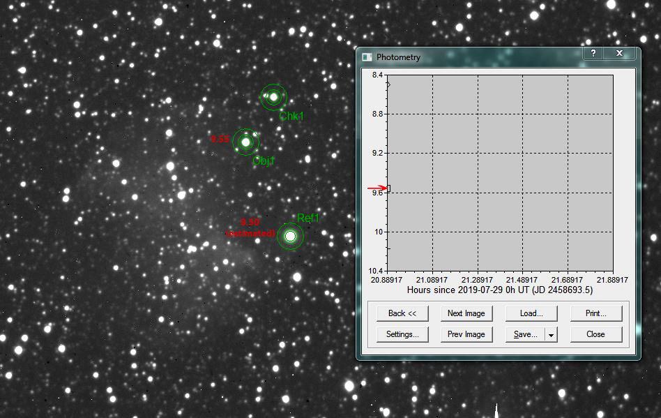
2- La sequenza di ripresa descritta in precedenza è stata poi focalizzata sulla variabile di Goldilocks, che nelle immagini conl’UHC, Neodymium e senza filtro mostrava apparentemente differenze non rimarchevoli di luminosità, mentre nel passaggio dal visibile senza filtri all’IR esplodeva in modo evidente in luminosità.In una parola, la variabile si accendeva allo spegnersi della nebulosa.Ho provato, non senza difficoltà, a fare una stima della magnitudine con Maxim DL , che sembra passare da 13.2 nel visibile a a 9.55 circa nell’IR (quest’ultimo dato è stimato a causa della impossibilità di avere una mag nell’IR tra 742 e 1000 per la stella di riferimento), ma coerente con la mag in J (9.42);H (8.38) e K (7.74), ed i valori di WISE, che la fanno scendere ulteriormente (6.91;6.56;4.92;3.83) . Comunque si va sulle 3.7 magnitudini di differenza tra le lunghezze d’onda da me considerate (mag integrata nel verde  a 550 nm per il visibile e intorno agli 850/900 nm per l’IR che è un riferimento attendibile sulla band pass del filtro e la  curva di risposta della camera). In proposito mi chiedevo se l’incremento di luminosità nell’IR fosse dovuto ad un inviluppo di gas  che nel visibile è nascosto da quello di gas e polveri di M27, tenuto conto che dovrebbe trattarsi di una gigante rossa pulsante.

Nell’animazione GIF allegata (6^ immagine) è condensato l’argomento del topic: la scomparsa di M27 e l’esplosione di luce di Goldilocks.Per inciso, nell’animazione è visibile anche la …sparizione di una stella luminosa nel visibile (probabilmente una stella con scarsissima emissione IR).Nella 7^ ed 8^ immagine sono mostrate le magnitudini della variabile ottenute sulla stella di riferimento.

                                       M27 and the Goldilocks variable: disappearance and appearance


On M27 there is now very little to say: it is one of the most famous, observed and photographed planetary nebulae of the northern sky. It was discovered by Messier in 1764 and is about 1360 light-years from the earth, it is of apparent magnitude 7.4, has an apparent diameter of about 8 arcominutes its shape resembles that of a dumbell-shaped spheroid (hence the name) and is seen along the perspective line of the equatorial plane, the kinematic age of the nebula would be 9800 years.The central star, like many planetary nebulae, it is a white dwarf.
Very few, however, are aware of two of its particular characteristics:

1- It hosts (among others) a variable to say the least strange for two reasons, the first that was discovered by the Czechoslovak amateur astronomer Leos Ondra not through the telescope and other optical instrument, but ... by looking at two magazines that showed an image on the cover in color of M27: the June 1990 number of Astronomy, and that of autumn of the same year of Deep Sky.Ondra realized that a star on the cover of the first magazine did not appear in the one of the second one. Astrometric and photometric works were after carried on, which confirmed to be a long-term variable (214 days) of Mira type (red, massive stars and pulsating), which was given the name "Goldilocks variable". But it does not end here: the star is also classified as object 2 Mass for its signature in the near IR (J (1.25 μ; H, 1.65 μ and K, 2.17 μ). It is also present in the Survey WISE (3.4; 4.6 ; 12 and 22 μ) and is listed by Simbad as NSV 24959 at the coordinates: 19: 59: 29.72 + 22: 45: 13.0.


2 - While in the visible the nebula M27 shows its splendid colors, from blue to red, as can be seen in the first image attached, in the IR near below the micron it literally disappears, also thanks to the power of penetration of the IR in the envelope of gas and dust.

So in a short vacation in summer 2019 I wanted to experiment with these features of M27:

1- by performing CCD recordings of the entire nebula:
     a) in LRGB
     b) with UHC filter
     c) with Neodymium filter (Anti IL)
     d) without filters
     e) with IR Pass filter> 742 nm
The instrumentation used was a Schmidt Cassegrain Celestron 8 telescope reduced to f 6.3 and a Sbig ST 10 camera used in 1x1 binning.
In the image n1 the usual LRGB of the nebula with the Goldilocks variable is shown; in the second the one with the Astronomik UHC filter, in the third the one with a Baader Neodymium, in the fourth the one without filters, and in the fifth one with an Astronomik IR Pass 742. While the variations in the appearance of the nebula with the various filters are modest, the one between the visible image without filters and that in the near IR is dramatic, with the practical disappearance of the nebula itself.

2- The sequence of images described above was then focused on the Goldilocks variable, which in the images with the UHC, Neodymium and without the filter apparently showed not remarkable differences of brightness, while in the passage from the visible without filters to the IR exploded in an evident way  in brightness. In a word, the variable was switched on when the nebula died out. I tried, not without difficulty, to make an estimate of the magnitude with Maxim DL, which seems to go from 13.2 in the visible to about 9.55 in the IR (this last datum is estimated due to the impossibility of having a mag in the IR between 742 and 1000 for the reference star), but coherent with the mag in J band (9.42); H (8.38) and K (7.74), and the values of WISE, which bring it down further (6.91; 6.56; 4.92; 3.83). However you go on the 3.7 magnitudes of difference between the wavelengths considered by me (mag integrated in the green at 550 nm for the visible and around 850/900 nm for the IR which is a reliable reference on the filter band pass and the chamber response curve). In this regard I was wondering if the increase in brightness in the IR was due to a gas envelope that in the visible is hidden by that of gas and dust from M27, given that it should be a giant red button.
In the attached GIF animation (6th image) the topic of the topic is condensed: the disappearance of M27 and the explosion of light from Goldilocks. Incidentally, the animation also shows the ... disappearance of a bright star in the visible ( probably a star with very little IR emission). In the 7th and 8th images the magnitudes of the variable obtained on the reference star are shown.

Valter Arno-Software per Fotometria

valter.arno@virgilio.it

Nel corso degli anni, la curiosità verso tematiche di carattere astronomico e informatico, mi hanno portato ad ottenere prima un B.Sc e poi un M.Sc in astronomia. Sono convinto che la rivoluzione operata dai moderni rivelatori CCD abbia offerto la possibilità di affrontare, con successo, lo studio di target altrimenti impossibili per ottiche di modesta dimensione. La proliferazione di tali rivelatori, anche in ambiente amatoriale, ha permesso di condurre studi di fotometria stellare talvolta molto complessi. Tuttavia, a fronte di potenzialità osservative elevate, capaci cioè di fornire quantità di dati significativi, non sempre si leggono studi che contengano deduzioni finali che dovrebbero derivare dalle interpretazioni di quei dati. Tutto ciò è ancor più evidente, se si affronta lo studio di target molto complessi che richiedono ingenti calcoli per analizzare e interpretare i dati fotometrici. A tale scopo, nei due articoli qui riprodotti è presentato un software gratuito, sviluppato su base Windows-Excel, in grado di analizzare e interpretare dati fotometrici di campi stellari complessi che si osservano negli ammassi galattici aperti o associazioni stellari OB. Si richiede soltanto una precedente riduzione e standardizzazione degli osservabili strumentali al sistema UBVIc. Il primo articolo contiene una descrizione tecnica dettagliata del software applicata all’ammasso stellare IC2581, mentre il secondo descrive la applicazione, dello stesso, allo studio della associazione stellare CMaOB1. Il software può essere richiesto gratuitamente all’autore, seguendo le indicazioni presenti negli articoli ( in lingua inglese).

Revisiting the Canis Majoris OB1/R1 association and star forming region.

Valter Arnò

Abstract.

This work does not claim to bring new results or discoveries. its purpose is merely to illustrate some photometric techniques, that can be used to study OB stellar associations. It is shown that OB stellar associations, can be studied using the same techniques employed for open galactic clusters.

Introduction.

About 25 minutes east and 6 degrees north of Sirius, at the boundary between the constellations of Monoceros and Canis Majoris just below the Galactic Equator, a very interesting star-forming region can be observed. This region which contains the stellar association CMaOB1, is located at galactic coordinates 220° < l < 226° and -3.4°< b < +0.7°. As in the neighbouring Monoceros OB1, the environment of CMaOB1 shows several features that indicate a region of recent star formation. Such features include: neutral hydrogen H I clouds, ionised hydrogen H II clouds, dark nebulae, emission nebulae, reflection nebulae and carbon monoxide molecular clouds. The most prominent features in the CMaOB1 region are represented by the interconnected structures Sh 2-292, 2-296 and 2-297. Over the last 50 years, this part of the sky has been intensively studied; both photometrically and spectroscopically. The latest study of Shevchenko has added new photometric data, so by mixing old and new data, we can revisit this association with the aim of determining some physical parameters. One of the best results of the extensive spectroscopic investigation of the Henry Draper catalogue, was the discovery that young O and B stars tend to cluster together as OB associations or young open clusters. It was also found that these stars are tightly condensed in a narrow band of a few hundred pc, across the mid-plane of our Galaxy. With the exception of a few runaway stars, observations clearly show that OB stars form and spend their lives in these particular regions of the Galaxy. Evidently, population I stars form where material and physical conditions are suitable for their construction. Today, we know three types of associations: OB, R and T. These acronyms identify concentrations of OB-type stars, reflection nebulae and T-Tauri type stars. The OB stellar associations are low-density groups of luminous and very hot stars with very short lifetimes. Due to their low density, typically 0.1 M_⊙ pc⁻³, these associations are weakly bound by gravity, so they cannot be held together for a long time. [1] As extremely young objects, the OB associations are always observed in the presence of the environment from which they formed. This means environments rich in: bright nebulae, dark nebulae, reflection nebulae and CO molecular clouds. As a rule, an OB association also contains T Tauri stars so they are also T associations; although the reverse is not always true. Due to their large Strömgren spheres, the presence of high concentrations of O-type stars strongly influences the interstellar medium (ISM). [2] [3] [4] On short timescales, O-type stars emit abundant fluxes of ultraviolet photons with wavelengths ≤ 912Å, together with X-rays and wind-driven mass losses ranging from 10^-7 M⊙ yr-1 to 10^-9 M⊙ yr-1. [5] Today we know that practically all stars brighter than are losing mass through their stellar winds. [6] The speed of these stellar winds is very high. Observation have revealed that the speed of the stellar wind emitted by an O5V star is, on average, about three times higher than that of a B0V star. More generally, going from spectral classes A to O, the speeds of the observed stellar winds lie in a range from ≃ 200 kms^-1 to ≃ 3000 kms^-1. [7] Such powerful stellar winds push away ionised gas and dust surrounding the O stars and this contribute not only to the formation of arc-shaped emission nebulae, but also, to carving out a vacuum bubble around these stars. The presence of ionised nebulae and strong stellar winds in the environment, can prevent the detection of faint reflection nebulae and thus the R association. The reflection nebulae are the result of the presence of very fine dust grains around stars. The size of these dust grains is about 500 nanometres. So, they are perfectly able to scatter short wavelengths more effectively than long wavelengths producing, in this manner, the typical blue haze characteristic of reflection nebulae. The reflection nebulae are illuminated by stars with spectral classes later then B0. Despite being very luminous to produce detectable reflection nebulae, these stars do not have sufficient ultraviolet fluxes to produce emission nebulae. In addition, the interaction between medium and late type B stars with the ISM is less powerful respect to O-type stars. Therefore, it is clear that within associations containing very few O-type stars and many B-type stars, the morphology of the environment from which they formed is better preserved. [8] The sizes of the OB associations can be considerable and, in some cases, can reach a radius of about 200pc. Because of their large size, the density of O and B stars is almost always low. Thus, from an observational point of view, an OB association appears as a sparse group of O and B stars. It is often difficult to separate the physical members of an association from the background stars, but it is relatively easy to determine their presence. To detect unusual concentrations of OB stars in a particular part of the sky, it will be sufficient to obtain images of the target field using two photometric filters such as U and V. A subsequent comparison of the images, will allow us to easily detect the stars for which the U magnitude is brighter than the V magnitude. The probability that the objects selected with this technique could be stars of spectral types O and B, is very high.

The CMaOB1 association a bit of history.

The first who noted the unusual concentration of B-type stars in the region of Canis Majoris, was Viktor Ambartsumian about 70 years ago. He named this concentration I Canis Majoris and defined this unusual aggregation of early type stars as a system of O-B2 stars with a common origin, whose spatial density is greater than the average local field density of these class of stars. [9] [10] Today we know this concentration as: CMaOB1, see figure 1.

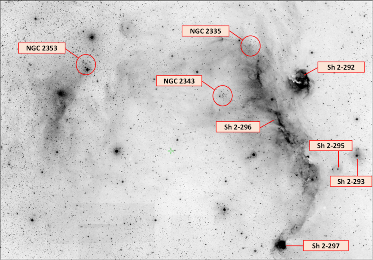
Figure 1 – DSS2 Red of CMaOB1/R1 semi-ring appearance.

After Ambartsumian, many other researchers turned their attention on this part of the sky. S. van den Bergh studied the distribution of reflection nebulae in this region which may or may not be associated with individual stars. [11] R. Racine reported photometric and spectroscopic observations of several individual stars. [12] J.J. Clarià planned an extensive photometric and spectroscopic study involving 247 stars. [13] [14] [15] Since the largest emission nebulae of CmaOB1 form a kind of semi-ring and this semi-ring also coincides with an expanding shell, W. Herbst and G.E. Assousa hypothesised that the whole complex could be a supernova remnant SNR, which in turn, triggered the star formation. [16] W. Herbst, R. Racine and J. Warner obtained UBVRIJHKL photometry and MK spectral types for stars illuminating the main nebulae in the region, including the Herbig AeBe emission line star HD 53367 and Z CMa. [17] During 1999, V. Shevchenko and co-workers, performed a new extensive photometric and spectroscopic study in this region between: 6^h 57^m < RA < 7^h 04^m and -9° 57’ > Dec > -12° 27’ involving 165 stars. [18] More recently the distribution of massive OB stars in and around CMaOB1 was studied by N. Kaltcheva and W. Hilditch, while J. Gregorio-Hetem summarised all our knowledge about CMaOB1. [19] [20] The most recent study was carried out by B. Fernades and co-workers during 2019. The authors have extensively studied the morphology of Sh 2-296, its relation to CMaOB1 and other nebulae, with particular attention to the 3 massive runaway O-stars present in this region: HD 57682-O9.2IV, HD 54662-O7V and HD 53974-B2I. [21]

Distance determination of CMaOB1 from 1966 to date

The determination of the distance modulus of CMaOB1 in the years to date is summarised in the next table 1, which brings together all the photometric investigation.

Table 1 – Estimated distance of CMaOB1.

Observed and intrinsic values

A photometric survey, usually consists of a long list of observations in terms of magnitudes and colours. So, if we use for example the UBV system, our observations could be expressed as: . However, as we know, the observables must be corrected for the effects due to extinction and reddening. Considering together the old and new UBV photometric surveys, we have a considerable amount of photometric and spectroscopic data. With these data we can obtain intrinsic values following different paths. We can use the photometric method, the spectroscopic method or both. It should be noted that, the photometric method requires some calculations, while the spectroscopic method allows intrinsic values to be obtained directly from empirical tables, see appendices A and B.

Obtaining the intrinsic colours using the Q method

W.W. Morgan and H.L. Johnson introduced, in the second half of the 20th century, the following quantity which is a parameter independent of reddening:. Furthermore, Morgan and Johnson also determined an empirical relationship between the value of the Q parameter and the spectral type as shown in the following Table 2. [22]

Table 2 – Q values and intrinsic colours for early type main sequence stars.

The intrinsic colours in Table 2 are still those reported by Johnson in 1958, although the currently accepted values are slightly different. The Q method allows us to select certain spectral classes or even spectral intervals from a variety of apparent measurements. The process of calculating and hence , for early type stars, with the Q method is iterative. This means that one proceeds by successive approximations. For these calculations, the following 3 equations must be considered:

The first step, in calculating each individual Q value, happens starting with equation (1) with a value for the ratio of the colour excesses . In the next step, the value of is obtained using equation (2) and hence Now, the ratio of the colour excesses is redetermined using equation (3). The whole process is repeated again using this last new value for the ratio of the colour excesses. Two iterations are usually sufficient as the values, from the second and third iterations, are in complete agreement. The Q method is only applicable to the early type main-sequence stars and therefore to stars belonging to the luminosity class V. We can apply this method, with some precautions, also to luminosity classes close to the main sequence, such as giant stars of luminosity class III. The Q method cannot be used for the luminosity classes II, Ib, Iab, Ia and Ia-0 which must be dereddened using the spectral type vs. intrinsic colour tables, see Appendix A table A1 and A2. The Q method can be easily implemented using an Excel spreadsheet. This advantage allows large amounts of data to be analysed very quickly.

Intrinsic colours from spectral classification

Another way to obtain intrinsic colours is possible considering only the spectral classification. In this case, the desired values can be deduced by consulting data published by various authors for instance: M.P. FitzGerald, C.W. Allen or Th. Schmidt-Kaler. [23] [24] [25] In Appendix A and B are given those of Schmidt-Kaler. Using such tables, one can obtain the intrinsic values , as a function of the spectral type and luminosity class. This means that each individual reddening and magnitude can be obtained through the following expression:and with R = 3. To make this clear, let's take an example. The star HD 51542 is an early type main sequence star of spectral class B3V (This classification is taken from the work of J.J Clarià to which we shall remain faithful, even if today Simbad reports for this star B2/3 III). This star shows the following reduced and standardised apparent values: , , . In Appendix A, table A1, we read for the spectral class B3 and luminosity class V, the intrinsic value . From this value we can calculate individual reddening and magnitude as follows: and . The Q method and the spectroscopic method may give slightly different values when applied to the same object.

Individual absolute magnitudes and distances

Unfortunately, reddening, intrinsic colours and corrected visual magnitudes, are not sufficient to determine individual distances. Each individual distance modulus is obtained through the difference , where M_V is the absolute magnitude. Therefore, to determine each individual distance, a relationship between a chosen unreddened colour index or and the absolute magnitude M_V, is required. Since we are considering an association of luminous and very hot OB stars, to define our relationship it is more convenient to use the colour index rather than the colour index. The reason for this latter choice will be immediately clear observing, in Appendix A Table A1, the trend of the colour index especially for stars belonging to the O spectral classes. In table A, we see how a same value of the colour index is shared by different spectral classes. For example, O6, O7 and O8 share the same value of i.e. -0.32. There is no such coincidence with the index! So, the relationship we are looking for, can be easily obtained using an Excel spreadsheet as shown in the next Figure 2. The absolute magnitudes and intrinsic colours in the left panel of Figure 2 come from the data of Schmidt - Kaler 1982.

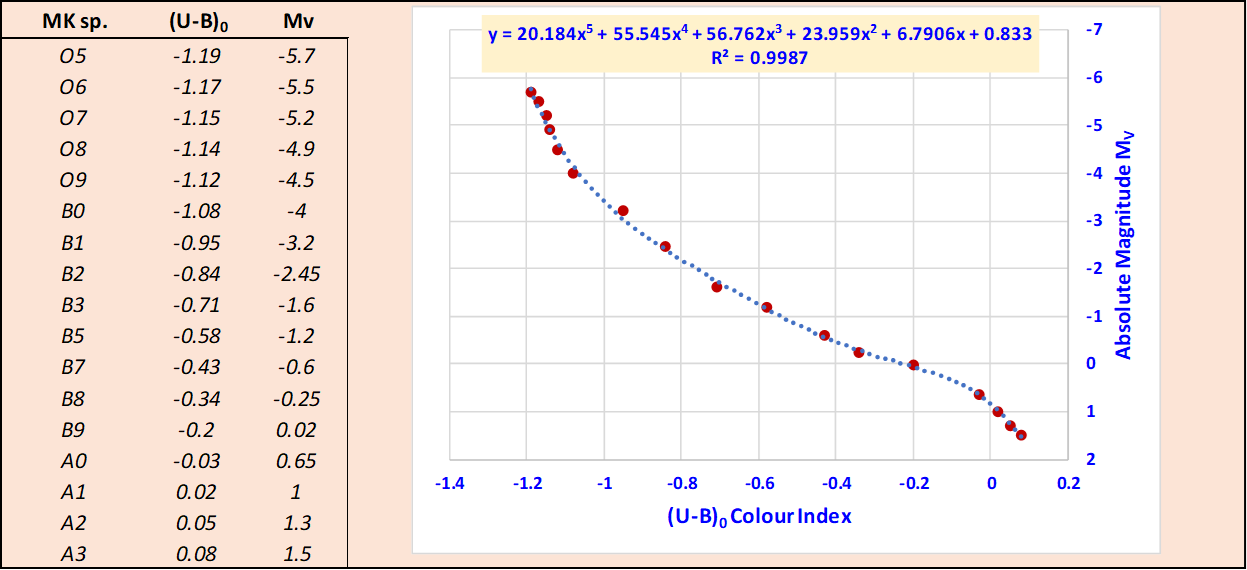
Fig. 2 The 5^th order polynomial relation between M_V and the colour index for population I early type stars.

The relation that give us each individual absolute magnitude M_V for stars of luminosity class V, as a function of each individual unreddened value can be written as follows:

(4)

With a value for R² = 0.9987, which indicates the goodness of the regression model. The field of application of equation 4 is: ≤. Using the results of the previous equation (4), we can obtain each individual distance modulus through the expression With an identical procedure, we can calculate each individual absolute magnitude and distance for luminosity class III, following the 5th order polynomial equation (5).

(5)

With a value for R² = 0.9992. The field of application of equation 5 is: .

Looking for the young massive and luminous OB stars.

In order to study an OB stellar association from a photometric point of view, we have to find a way to separate their likely members from the background stars. Therefore, while searching through the photometric data, we need to extrapolate only those values correlated with the objects we are interested in. Since the OB associations are composed of very young massive early type stars, in this study we will limit our search to stars belonging to the spectral classes in the range O5-B5. This means stars with absolute magnitudes in the range , for luminosity class V and between for luminosity class III. Stars whose emissions are perfectly capable of exciting or ionising the ISM surrounding them. The average distance modulus of CMaOB1 considering all the previous studies (see Table 1), converges to a value of 10.15 mag., i.e. about 1071 pc. Given this average distance, we expect the resulting V magnitude for the selected stars to be in the range . Where V is the apparent visual magnitude under ideal conditions, i.e. ignoring the effects produced by ISM. For the reasons just given, we will apply some selection criteria when examining all photometric data. We will consider only stars belonging to luminosity classes V and III with visual magnitude not fainter than V = 9.50 and with a Q value ≤ -0.44. The Q value is useful to exclude spectral classes later then B5 from our search (see Table 2). Unfortunately, the Shevchenko study does not provide a luminosity classification and most of the studied stars belong to spectral classes later than B6. More than 25 years separate the work of Clarià from that of Shevchenko. After so many years, the data obtained by the two authors require, as a first step, a comparison of the stars in common, this in order to verify the accuracy of the measurements. In the two studies there are 15 stars in common and Figure 3 shows this comparison between the measurements of Clarià and Shevchenko in terms of V and

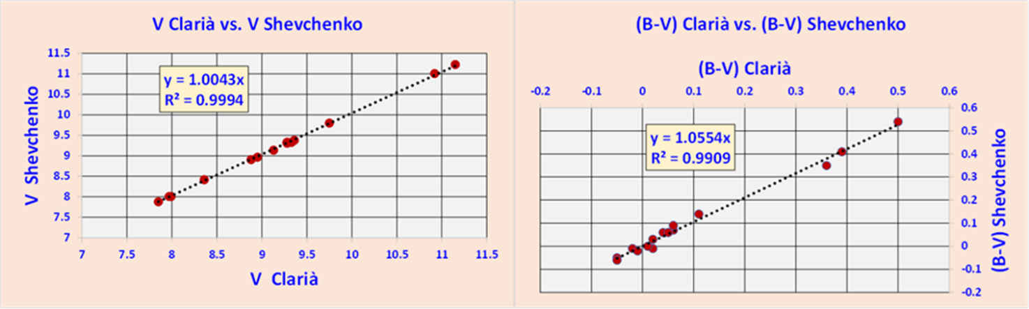
Figure 3 Comparisons of stars in common between the two studies.

As can be seen, there is no evidence of major systematic differences for common objects between the two works and all the points fit according to a Y=X type law, with very small discrepancies. Individually, the values obtained from the previous work can also be compared with those contained in the General Catalogue of Photometric Data. [26] Once it has been established that the two studies are comparable, one can proceed to determine each individual un-reddened value from the observables using the Q method or, alternatively, the spectral classification if available. It should be noted that the Q method provides continuous values, whereas spectral classifications provides quantified values.

Photometric diagrams

The photometric diagrams are very useful. A careful analysis of their appearance can provide valuable information. Figure 4 shows the two-colour diagram vs. and the colour-magnitude vs. diagram combined in two panels. The left panel of figure 4, shows the combined data from the two studies. The right panel contains the results of the analysis performed using the Q method, adopting the above selection criteria. Having chosen to select only stars earlier to the spectral class B5 that means Q ≤ -0.44, one can clearly see the presence of two stellar groups with different reddening in the left panel of figure 4. These two stellar groups, can be easily separated through the reddening line . The group above this reddening line which shows differential extinction, is the only one we are interested in. This group consists of stars earlier than the B5 spectral class with surface temperatures between 16000 and 44000 T_eff [K°]. Given the high temperatures and the consequent high luminosities, it is easy to deduce that these stars are perfectly able to excite and ionise their surroundings. Looking at the right panel of figure 4 one can see the absence of OB stars below a very precise left boundary. This boundary also represents the lower luminosity locus of the distribution of the points. Note that the lower luminosity locus reproduces, quite well, the zero-age main sequence for O5-B9 stars (blue curve) and this suggests the existence of a group of early type stars located, more or less, at the same distance. Obviously, as we shall see later, not all stars shown on the diagram will be members of the association. This also explains, along with other various effects such as evolutionary phenomena, rapid rotators and probably large number of binaries, the considerable dispersion of the points to the right of the lower luminosity locus.

The reddening vs. distance modulus diagram

Figure 5, shows the reddening plotted against the distance modulus for all the stars selected with the Q method. From this diagram we see that the majority of the early O5-B5 type stars, are clustered at a distance modulus between 9.5 and 11 mag. with a mean concentration around 10.25 mag. Moreover, we see that this group is subject to a variable differential extinction in the range This effect is certainly due to the presence of bright and dark nebulae at that distance. Indeed, the present distance modulus of the molecular complex Sh 2-292, 2-293, 2-295, 2-296, 2-297 is estimated to be about 1.15 ± 0.14 Kpc., corresponding to = 10.24 mag. [27]

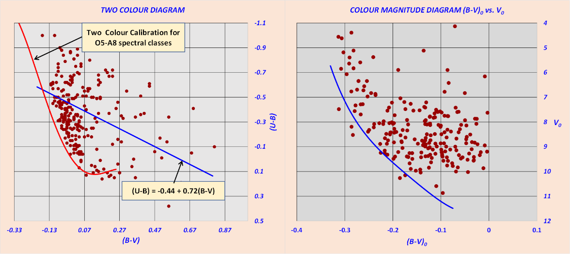
Figure 4 The two colour and colour magnitude diagrams.

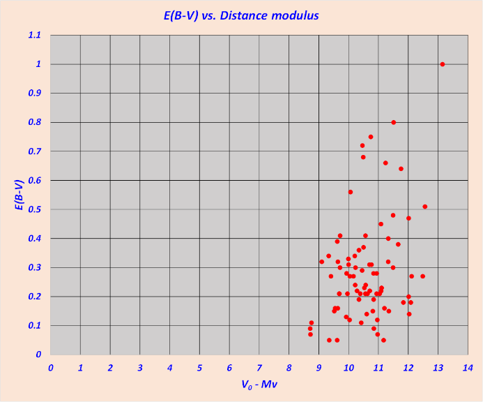
Figure 5 vs. for all stars confined above the line

Membership issue

Using the Q method and photometric diagrams, we were able to establish the existence of a significant number of early type stars at a distance compatible with the molecular complex, represented by the nebulae Sh 2-292, 2-293, 2-295, 2-296 and 2-297. The overall selection we made using the Q method, identified 72 stars belonging to the O5-B5 spectral range. But which and how many of these stars can be considered members of the CMaOB1 association? Establishing membership is never a simple matter. This is mainly due to the difficulty of identifying and separating the physical members of the OB association, from the stars belonging to the stellar background. In principle, membership analysis can be carried out using different criteria such as: kinematic, statistical, photometric and spectroscopic. Since we have only photometric and spectroscopic data, the membership was investigated using these last two criteria.

The photometric criterion

Assuming a coeval star formation, the photometric criterion states that all stars that can be considered as probable members of the association must fall on a well-defined evolutionary sequence. Obviously, this evolutionary sequence must be compatible with the age of the association this because, in conclusion, the colour magnitude diagram is an isochrone corresponding to the age of the association. Substantially, the positions of the probable members on the two-colour and the colour-magnitude diagrams, must be compatible with their spectral classification and photometric distances. The stars located far from the field of interest that show inconsistent photometric distances can also be considered as non-members. More generally, all stars that do not meet the above criteria may be considered non-members. The above criteria work well when the field stars have different ages, reddening and distances respect to the OB association. Therefore, according to the previous definitions, we have to check, for each considered star, the consistency of its position on the sky, with its position in the photometric diagrams and the evolutionary status suggested by its spectral classification. To check the position on the sky, was used the ALADIN application by loading the HD catalogue. In brief, these comparisons can be made using the vs. diagram, the vs. diagram, the spectroscopic classification and the positions on the sky as shown in Figures 6, 7 and 8. In both photometric diagrams of figure 6 and 7, the zero-age main sequence has been placed at a mean value derived from the Q analysis. By way of example, in these figures are analysed the positions of two stars considered to be probable members. The first star HD 53339, is classified B3V while the second star, HD 53456, is classified B0V. As can be seen in figure 6 and 7, both stars are clearly identified as main sequence class V. In addition, they also fall within the range defined by the Walker’s criterion for main sequence stars. [28]

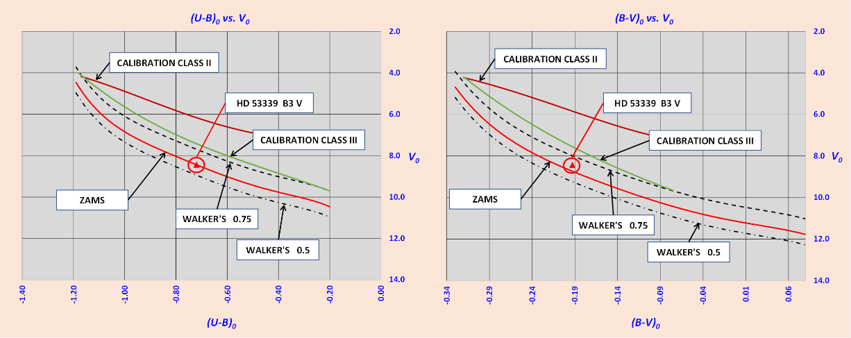
Figure 6 HD 53339 B3 V is identified as main sequence star on both two-colour diagrams.

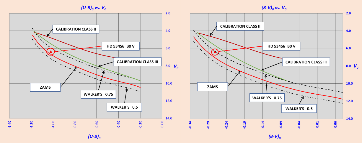
Figure 7 HD 53456 B0 V is identified as main sequence star on both two-colour diagrams.

The Walker’s criterion implies that a member should have a distance modulus no more than 0.5 magnitudes from the mean modulus and the duplicity should not brighten a star by more than 0.75 magnitudes, always from the mean modulus. The Walker’s criterion is only reliable for main sequence class V stars. Figure 8 shows the positions of HD 53339 and HD 53456 on the sky.

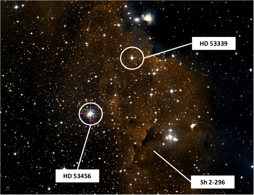
Figure 8 the identification of HD 53339 B3V and HD 53456 B0V on the field of Sh 2-296.

Spectroscopic criterion

As in the previous case and for a given individual star, the spectroscopic criterion is based on the determination of its spectral type and luminosity class. A comparison between spectral and photometric information, can give us an idea of the evolutionary status of that star. Therefore, if a star is located in a different evolutionary status from the expected position on the colour-magnitude diagrams, then that star is not a member.

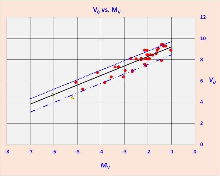
The V₀ vs. M_V diagram

The probable membership of the 72 OB stars identified using the Q method, was further investigated using the vs. diagram as shown in figure 9. Based on the above requirements and due to the application of the photometric and spectroscopic criteria, 36 stars were discarded. The vs. diagram of figure 9, shows the remaining 36 OB stars that can be considered as probable members of CMaOB1.

Figure 9 – The V₀ vs. M_V diagram.

This group has an average distance and it contains 34 class V main sequence stars and 2 class III giants. The vs. diagram in figure 9, prove the existence of a linear relation between and for the stars listed in the following table 3. This linear relation implies that we are considering a physical group of stars. In the same diagram are also shown the limits of the Walker criterion using the two dotted and . The following table 3 contains the list of probable members.

Table 3 – List of CMaOB1 probable members.

Probable members on the two-colour diagram and variable differential extinction

The next Figure 10 shows, on a two-colour diagram, all the stars listed in Table 3 selected, as probable members of CMaOB1. The thirty-six probable members are shown together with their O5-B5 reddening lines. In this plot we can also see that the probable members are reddened by two different effects.

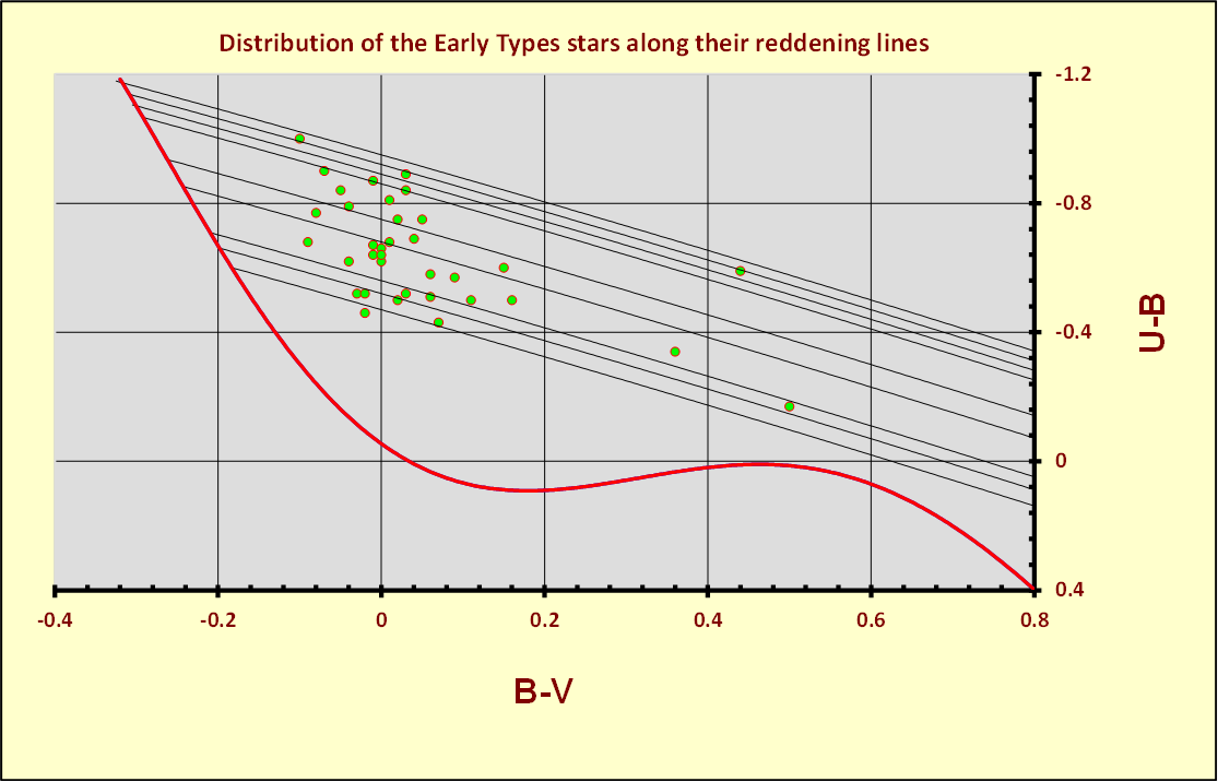
Figure 10 – The thirty-six probable members on the two-colour diagram and reddening lines O5-B5.

The first, more general effect, is due to the distance of the entire group of stars from us. That is the distance of the stars lying on the blue-most envelope of the distribution, with respect to the intrinsic two-colour calibration (red curve). The second effect is more local. It is due to the environment surrounding the young OB stars. Regarding this last effect, we can clearly see how starting from the blue-most envelope of the distribution, all the stars tend to spread out along their own reddening lines. This should not be surprising, as such a phenomenon would be expected in the environment in which an OB stellar association forms and evolves. Under these conditions, the absorption due to the distance at which the group of young OB stars is located is supplemented by a further differential absorption within the OB association. The latter phenomenon it is due to the passage of light through the material - still present - from which the young OB stars were born. However, this also means that the stars considered as probable members and listed in Table 3, must be studied taking in consideration also this aspect. To Study the OB associations still embedded in their nurse regions, we must first determine the value of the differential extinction and then the value of . In Figure 11 we can see how the determination of the parameter can be obtained using a specific application that allows us to make such measurements.

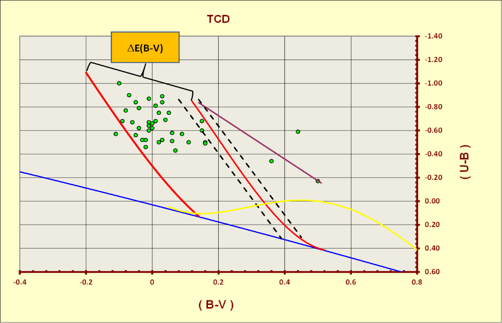
Figure 11 – Determination of for CMaOB1 probable members.

In presence of a large amount of differential extinction, each individual value of , must be obtained considering all the reddening lines that do not have double intersections with the intrinsic colour calibration. This condition is fulfilled for a value of the Q parameter less or equal to -0.38. Thus, following Golay M., each individual value is obtained as shown in with equation (6), where X = 0.72. [29]

With the individual intrinsic values for the probable thirty-six members of CMaOB1, we can construct the vs. and the vs. diagrams. With these diagrams awe can derive the distance of this group of stars using the Zams fitting procedure, on both diagrams, as can be seen in the following Figures 12 and 13.

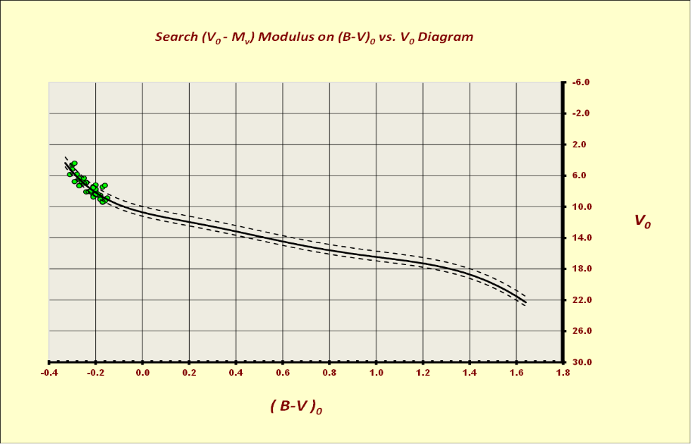
Figure 12 – Fitting distance on the vs. plane.

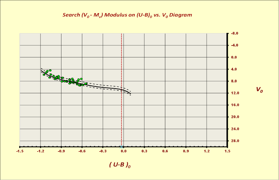
Figure 13 – Fitting distance on the vs. plane.

The next step is to move from the observational to the theoretical plane as can be seen in Figure 14. In the theoretical plane, we see that our sample of probable members is represented by stars whose mass distributions fall in a range between 4 and 40 solar masses. The turn-off point is well constrained using the Bertelli isochrones for logarithmic ages between 6.6 and 6.7. An age between 3.98 x 10⁶ and 5 x 10⁶ years. [30] Furthermore, the theoretical diagram shows that there are at least 8 stars in this group that reach a bolometric magnitude greater than M_bol = -6. Most likely, the future changes in the morphology of the environment of CMaOB1, will occur through the action of the stellar winds produced by these stars.

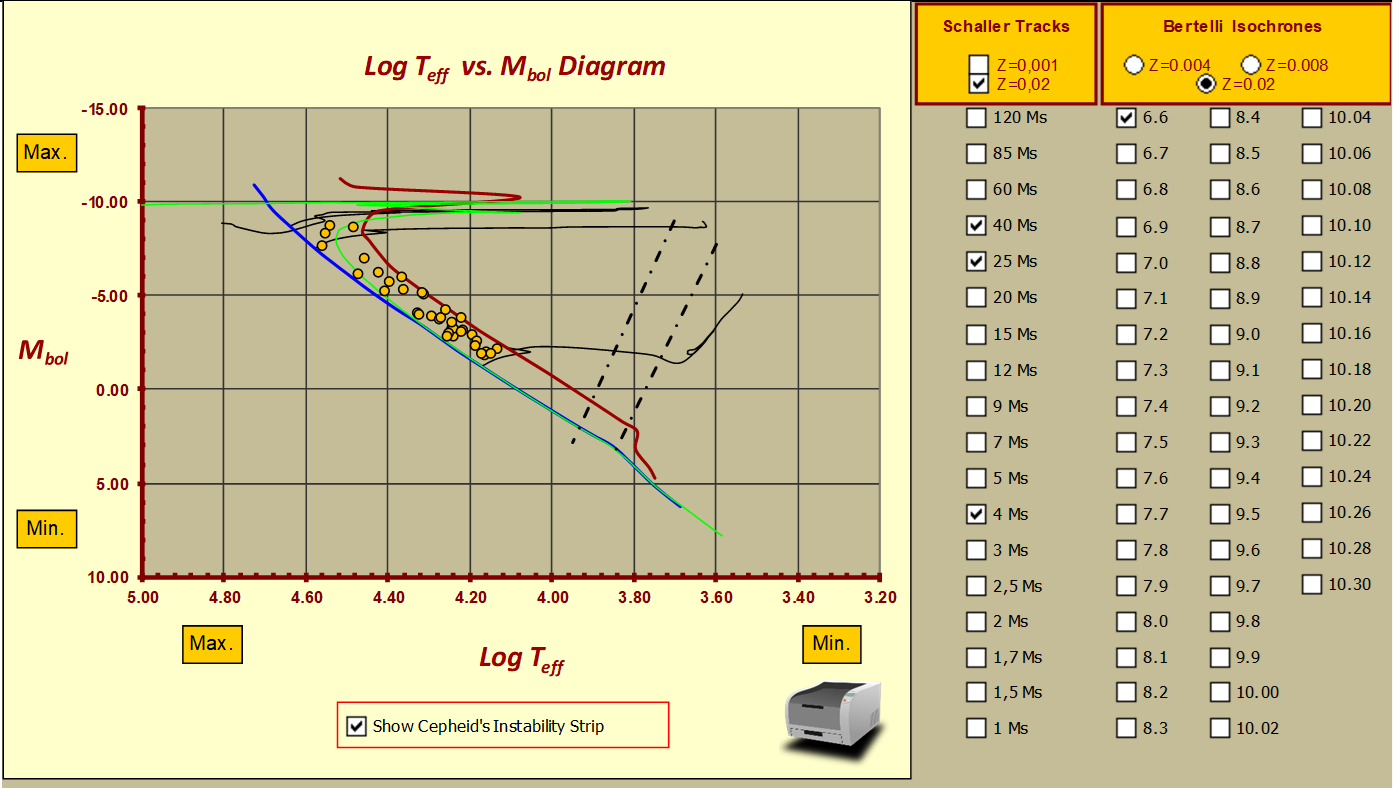
Figure 14– Probable members on the theoretical plane Log T_eff vs. M_bol.

Figure 15 summarises the final distance modulus for our O5-B5 sample that turns out to be: 10.105±0.07 mag. or 1049 pc. Our results seem to be in good agreement with the most recent determination of the distance modulus of CMaOB1 obtained by professionals see Table 1. The age result, in figure 15, is shown using the Excel’s scientific notation, so means .

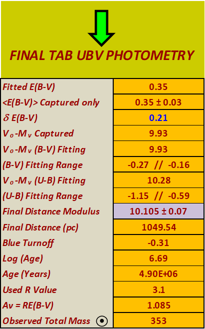
Figure 15 – Final data for probable members of CMaOB1.

Brief considerations on population of the HRD instability strips of our sample of OB stars

It may also be interesting, for a possible study of variability, to observe that at least 30 stars out of 36 in our sample, fall in two well-known instability stripes on the HR diagram. The two instability stripes concern the  Canis Majoris and the SPB slowly-pulsating B stars variables. See next figure 16.

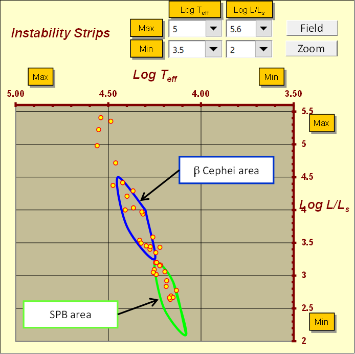
Figure 16 –  Canis Majoris and SPB instability strips.

In the case of proven variability of some probable member and since we have derived the absolute magnitude considering these stars as a probable members of CMaOB1; it would be possible to compare our absolute magnitude determination with that derived from the equation 7 of Blaauw and Savedoff.

Where, M_V is the absolute magnitude and P is the period of variability in hours. [31] [32]

Summary

The content of this work focuses on OB stellar associations and it is shown that, despite their sparse nature, OB associations can be studied with the same approach as open clusters. Among other things, a no less important issue is discussed. This issue, concerns the methods to be used to assess the membership of such dispersed objects in the sky.

References

1. Wright N.J., et al., OB associations, https://arxiv.org/pdf/2203.10007 (2022)

2. McCullough R.P., Publ. Astron. Soc. Pacific, 112, 1542 (2000)

3. Strömgren sphere, https://en.wikipedia.org/wiki/Str%C3%B6mgren_sphere

4. Oregon State University Strömgren sphere, http://homework.uoregon.edu/pub/class/321/sspher.html

5. Kobulnicky H.A., Astronomical J., 128, 73 (2019)

6. Snow T.P., Astrophysical J. Supp., 32, 429 (1976)

7. Bernabeu G., et al., Astronomy & Astrophysics, 226, 215 (1989)

8. Herbst W., Star Clusters IAU Symposium 85, 33 Dordrecht D. Reidel Publishing (1980)

9. Ambartsumian V., Publication Armenian Academy of Sciences, (1948)
   http://vambartsumian.org/lib/pdf/stellar_associations.pdf

10. Ambartsumian V., Publication Armenian Academy of Sciences, (1954)
    http://vambartsumian.org/lib/pdf/multiple_systems_of_trapezium_type.pdf

11. van den Bergh S., Astronomical J., 71, 990 (1966)

12. Racine R., Astronomical J., 73, 233 (1968)

13. Clarià J.J., Boletim de la Asociacion Argentina de Astronomia, 16, 27 (1970)

14. Clarià J.J., Astronomical J., 70, 1022 (1974a)

15. Clarià J.J., Astronomy & Astrophysics, 37, 229 (1974b)

16. Herbst W., & Assusa G.E., Astrophysical J., 217, 473 (1977)

17. Herbst W., Racine R., Warner J.W., Astrophysical J., 223, 471 (1978)

18. Shevchenko V.S., et al., Monthly Notices Roy. Astron. Soc., 310, 220 (1999)

19. Kaltcheva N.T., & Hilditch R.W., Monthly Notices Roy. Astron. Soc. 312, 753 (2000)

20. Gregorio-Hetem J., Handbook of Star Forming Regions Vol II, Astronomical Society of Pacific (2008)

21. Fernandes B., et al., Astronomy & Astrophysics, 628, 44 (2019)

22. Johnson H.L., Lowell Observatory Bulletin, 4, 37 (1958)

23. Fitzgerald M.P., Astronomical J., 71, 990 (1966)

24. Allen C. W., Astrophysical Quantities, Athlone Press London (1973)

25. Schmidt-Kaler Th., Landolt Bornstein Group IV, Vol. 2 Stars and Star Clusters, Springer (1982)

26. Mermilliod J.C., et al., General Catalogue of Photometric Data,
    https://gcpd.physics.muni.cz/cgi-bin/photoSysHtml.cgi?0

27. Blitz L., Fich M., Stark A., Astrophysical J. Supp. 49, 138 (1982)

28. Walker G.A.H., Astrophysical J.,141, 660 (1965)

29. Golay M., Introduction to Astronomical Photometry, D. Reidel Publishing Company (1974)

30. Bertelli G., et al., Astronomy & Astrophysics Supp., 106, 275 (1994)

31. Blaauw A., & Savedoff M., Bulletin Astronomical Institute Netherlands, 12, 69 (1953)

32. Flugge S., Handbook der Physic Vol. II section 25, 398 Springer-Verlag (1958)

Appendix A

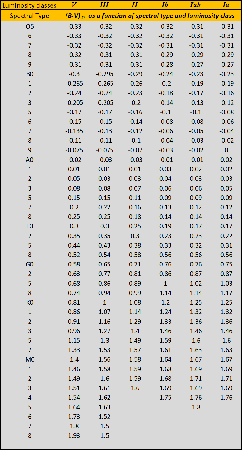
Table A1 – (B-V)₀ colour index as a function of spectral type and luminosity class from Schmidt-Kaler 1982.

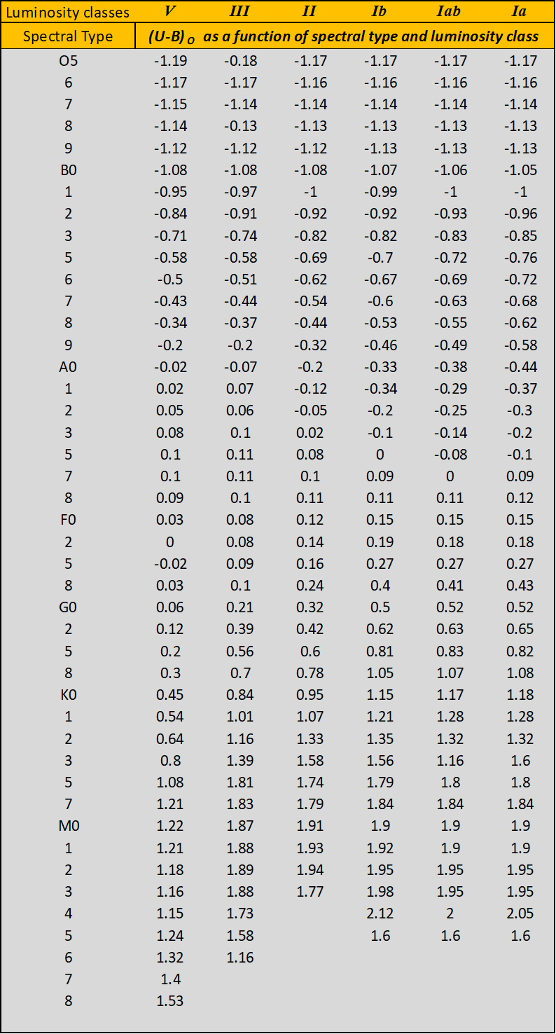
Table A2 – (U-B)₀ colour index as a function of spectral type and luminosity class from Schmidt-Kaler 1982.

Appendix B

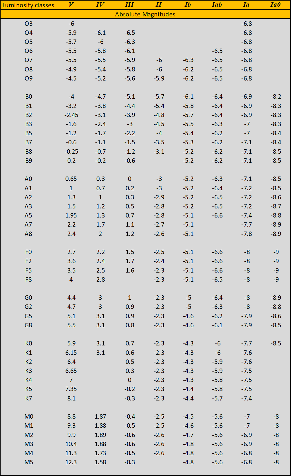
Table B1 – Absolute magnitude as a function of spectral type and luminosity class from Schmidt-Kaler 1982.

A tool for quickly reach UBVIc photometric scenarios of OB stellar associations and galactic open clusters.

Valter Arnò

Introduction.

This interactive tool performs the extensive calculations needed to analyse UBVIc photometric data for OB stellar associations and open clusters allowing also evolutionary models to be investigated and tested. the main objective is to obtain, in a very short time, the scenario resulting from a comprehensive photometric study, which can be the basis for subsequent and more detailed studies.

The software.

This tool can be used either for research or simply for educational purposes such as: classroom demonstrations and training of astronomy students. In order to transform Excel into a code suitable for studying open clusters, we need to implement a number of different algorithms, with the aim of using it as a code dedicated to this type of study. All this, without forgetting that this code works with well-standardised UBVIc data. This means that the reduction and standardisation of the instrumental data are two fundamental steps for the success of the subsequent photometric analysis. Using some spreadsheets, together with the standard techniques associated with photometric diagrams, Johnson H.L. & Morgan W.W. (1953) and Cousins A.W.J. (1978), we can analyse the observed data in order to obtain various parameters, such as: intrinsic colours, effective temperatures, distances, absolute and bolometric magnitudes, ages, metallicities, luminosity functions (LFs), present day mass functions (PDMFs) and many other data. [1] [2] The code comes with some default clusters for UBV and BVIc photometry, whose photometric values are taken from the Nasa-ADS technical literature. Default clusters are essential as they are supported by various hints and are useful to become familiar with the behaviour of the code. They have also been chosen to represent and cover all possible situations. Of course, the user can add and store their own data up to a maximum of 500 clusters for each type of photometry.

The observational data.

Although open clusters can be studied using a variety of photometric systems, this code focuses on the use of the UBVIc system, which is fairly common among amateurs. Regarding cluster members, our observational data are essentially apparent magnitudes and colours and several steps are required to convert observational quantities into effective temperatures and luminosities. Starting with the apparent magnitudes and colours, we need to correct for extinction and reddening effects and if the distance is known, we can obtain the absolute magnitudes. Furthermore, in order to compare our observations with theoretical stellar models, we must also take into account the fraction of the flux not detected by our observing window, using the so-called bolometric correction hereafter (BC) Heintze J.R.W. (1973). [3] It is only at this point that the conversion of the colours into effective temperatures, as well as the conversion of the absolute magnitudes into luminosities, becomes possible. The final step is to compare our data with theoretical tracks and isochrones. Of course, if we want to get significant results, the signal coming from our target must be free of noise. As we know, the light signal can suffer various losses due to the combined effect of our instrumental system, atmospheric absorption and interstellar absorption. Ignoring the first two, as they are handled by reduction and standardisation, let’s see how the code tries to evaluate the reddening due to interstellar absorption.

The average cluster colour excess <E(B-V)>.

Interstellar space is not empty. It is filled with rarefied gas and dust acting as filters. Therefore, apparent magnitudes and colours tell us nothing about the physical reality. The interstellar medium dims distant stars making them redder than their true colours. Astronomers call these effects as extinction and reddening. We can define extinction as the difference between the observed magnitude and the magnitude that would be measured if the interstellar medium were completely transparent. Similarly, we can define reddening as the difference between the observed and the intrinsic colour of a star. This difference is often called: colour excess. Let’s see how the code quantifies extinction and reddening. In the UBV system the there are two widely used colour indices: (U-B) and (B-V). The amount of the ultraviolet radiation emitted by a star is measured by the (U-B) index, while its temperature is measured by the (B-V) index. Using these indices, we can construct two fundamental diagrams for our purposes namely: the colour versus colour or two-colour diagram hereafter (TCD) and the colour versus magnitude diagram hereafter (CM). The TCD is particularly useful for obtaining both the average cluster reddening <E(B-V)> and each individual reddening for cluster members belonging to the early spectral classes O, B. Let’s see how. Figure 1 shows the Schmidt-Kaler (1982) un-reddened two-colour calibration, [4] i.e. the locus of the intrinsic colours (blue curve), shifted along the slope of the reddening line, hereafter RL (black line), until to the blue-most envelope of the cluster - in this case M36 - is reached (red curve). The amount of this shift represents the average cluster colour excess <E(B-V)>. This is a very delicate phase and the code requires the cooperation and judgement of the user to identify the blue-most envelope of the cluster on the TCD. The code can help the user to identify the blue-most envelope, by performing a scan of the intrinsic calibration along the slope imposed by the RL. Figure 2 shows the result of this scan for the southern cluster IC2581.

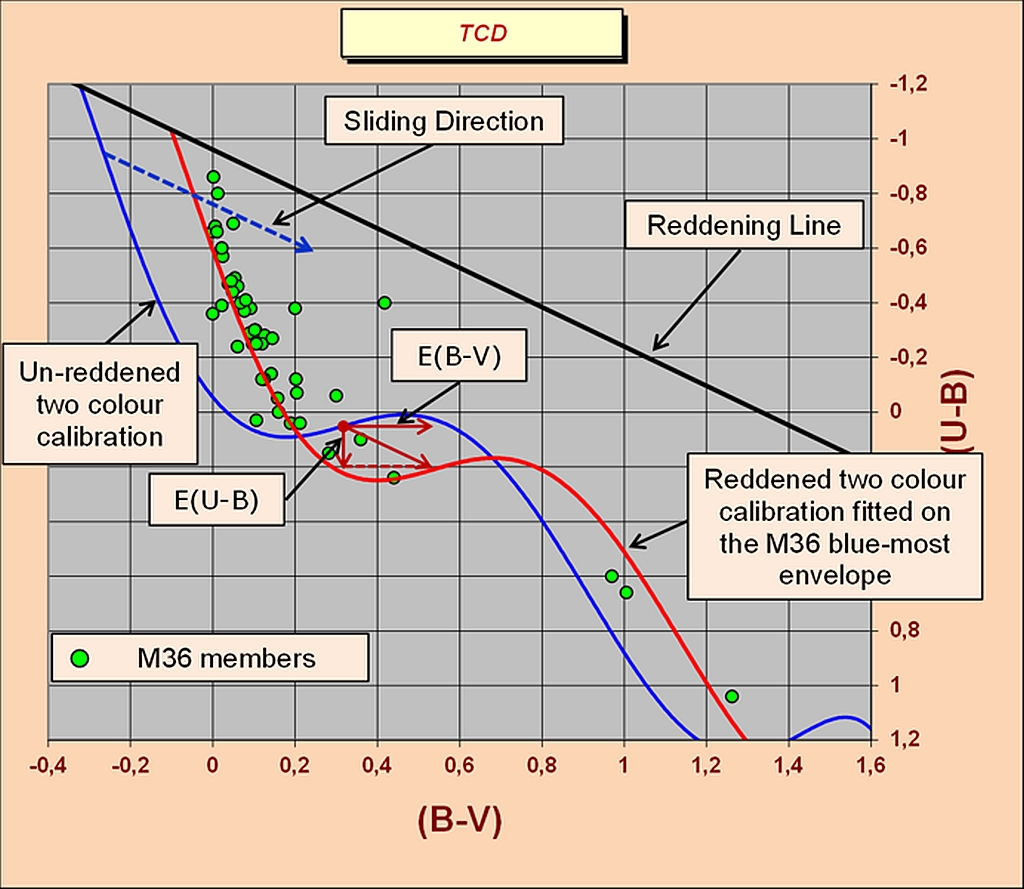
Figure - The sliding fit technique applied to M36.

The histogram clearly shows that the counts density changes between 0.38 and 0.43 E(B-V). The left slope of the histogram represents the boundary of the foreground reddening for IC2581. So, from an operational point of view, while we are sliding the un-reddened intrinsic calibration on the TCD, we need to find the best fit with the cluster array around this E(B-V) range.

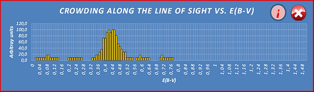
Figure - Finding the blue-most envelope for IC2581.

The scan performed by the code on the TCD is obtained by superimposing a rectangle of defined and constant area on the part of the intrinsic calibration representing the spectral classes O, B and early A. The pitch of the scan is very small, typically one hundredth of E(B-V). The capture rectangle is centred midway on the calibration and its size covers an equal capture area to the left and to the right of the calibration. Therefore, each star can be captured several times during the scan. For this reason, the unit reference of the ordinate of the histogram is arbitrary. After all, the purpose of the histogram is limited to highlighting the position of the blue-most envelope, i.e. the boundary of the foreground reddening. The shape of the empirical un-reddened calibration, drawn by Excel, is obtained through a 6^th order interpolating polynomial from Schmidt-Kaler (1982) tabular data. [4] The general expression for this calibration can be written as follows:

Where the Greek letters represent the regression coefficients while (U-B)₀ and (B-V)₀ the un-reddened colours. From a graphical point of view, the user must be aware that the polynomial regression curves provided by Excel are neither splines nor piecewise polynomials. For this reason, the Runge’s phenomenon cannot be avoided and some fluctuations may occur in the Excel graph.

Individual Intrinsic colours.

Returning to Figure 1, we see that the cluster array (green dots on TCD), is shifted to the right and down along a phat almost parallel to the RL with respect to the position of the un-reddened two-colour calibration (blue curve). This shift is due to the effect of the interstellar absorption. If we take into account this effect, we can also say that the distance between an observed point on the TCD and the intrinsic two-colour calibration gives the individual colour excess for that point. Obviously, each distance must be computed along the corresponding reddening line. In this way, we can also define each individual RL as the locus where we find, sometimes scattered, stars of the same spectral class with the same intrinsic colours, but subjected to different degrees of interstellar absorption. Now, as in the UBV system the RL slope is known for the stars of the early spectral classes O and B, it is possible to obtain the intrinsic colours of these stars. Strictly speaking, the RL is not just a straight line and can be well represented by the following quadratic expression:

While the ratio between colours excesses is:

In the previous equations, X is the RL slope and Y represents its curvature. The commonly accepted values of X and Y for the OB stars are: 0.72 for the slope and 0.05 for the curvature. However, Turner D. G. (1989) and (1994) expressed some criticism about these values. [5][6] Therefore, it seems that the determination of the intrinsic colours on the TCD, can substantially be reduced to a geometric issue. Moreover, since the analytical expression of the two-colour calibration is not definitely linear, it is clear that finding a common solution between the RL and the two-colour intrinsic calibration may involve some difficulties. However, to get out of this impasse, it is sufficient to observe that open clusters are young objects whose members are also young stars belonging to the spectral classes O, B, A. Therefore, the previous equation (1) can be reduced from a 6th order polynomial to a regression line by restricting the data interpolation of our intrinsic calibration to the spectral classes O, B and early A as follows:

Equation (4) simplifies considerably and allows us to obtain the intrinsic colours, at least for the programmed early-type stars in our open cluster. To do this is sufficient to construct various reddening lines connecting the observed positions with the intrinsic colour calibration equation (4), in order to read the coordinates of the intersection points. We just have to avoid the application of this method, where ambiguous solutions can occur due to multiple intersections between the reddening line and the two-colour calibration, as explained in Figure 3. Clearly, we can obtain an accurate determination of the intrinsic colours, if the slope of the RL is as different as possible from the slope of the two-colour calibration. Unfortunately, using UBV photometry only, this statement is not equally true for all spectral classes and astronomers have developed alternative systems for de-reddening medium and late type stars. For example, the BVIc system is ideal for de-reddening Cepheid and yellow stars. Dean W.W., Warren P.R. and Cousins A.W.J. (1978) have derived the reddening free locus of Cepheids using the (V-I) vs. (B-V) plane. [7]

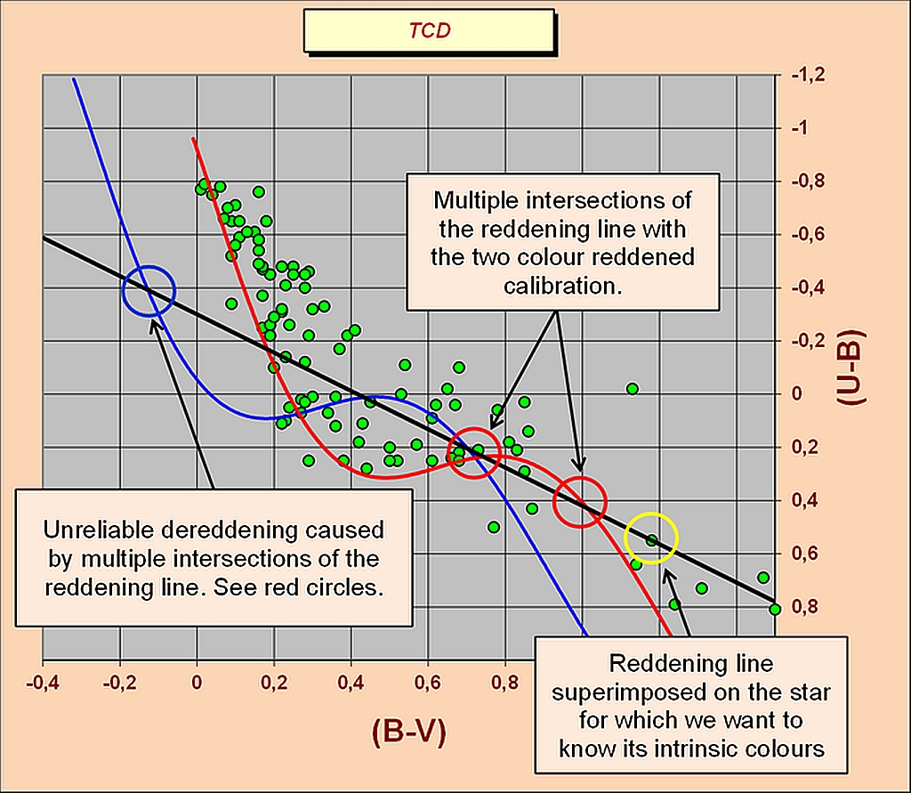
Figure - Unreliable de-reddening

The authors calibrated the zero point from photoelectric observations of stars inside clusters or associations, with well-known reddening values. They showed that using the (V-I) vs. (B-V) plane, the reddening slope and the reddening index can be represented by the following relationships:

and:

Where X is given by the ratio E(V-I)/E(B-V) for a star with E(B-V) tending to zero and (B-V) = 0, while E₀ is the colour excess that a star with (B-V) = 0 would suffer, when observed through the same amount of absorbing material. For BVIc photometry the normal ratio used by the code is: E(V-I)/E(B-V) = 1.25 Straižys V. (1992). [34] Furthermore, using the BVIc system and plotting the two-colour calibration with its corresponding reddening line on a (V-I) vs. (B-V) - (V-I) diagram, we will see that the slope of the RL is suitable for discriminating stars in the F5÷K1 spectral range, Pollacco D.L. (1989) and Pollacco D.L. & Ramsay G. (1992) see Figure 4. [8] [9] The data for the calibration in Figure 4 are taken from Cousins A.W.J. (1978). [2] Another way to estimate the reddening of a late type star relative to an early B0 type, can be evaluated considering that the value of X = E(U-B)/E(B-V) for intermediate and late type stars is significantly different, from an early B0 type star. According, to Schmidt-Kaler Th. (1961) or Fernie J.D. (1963), we can estimate the reddening for these stars defining the quantity  as follows:

Where the subscript SP means: spectral type. [10] [11]

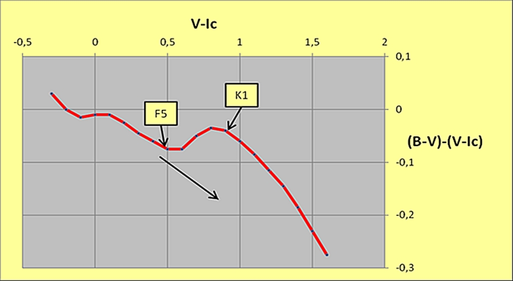
Figure - The (V-I) vs. (B-V)-(V-I) diagram.

Computation of the total absorption.

The total absorption in the visual magnitude V can be evaluated on the basis of the following expression:

Where A_V and A_B are the absorptions in V and B bands respectively. We can also define the observed quantities as follows:

Since E(B-V) = A_B - A_V equation (8) becomes:

By knowing the spectral types for a sample of stars in a cluster, the ratio R of total to selective absorption can be estimated, Turner D.G. (1976). [12] In practice, one uses the Johnson’s cluster method (1968), assuming that all stars in the cluster volume are equally distant from us (i.e. neglecting the depth of the cluster itself, which can be considered tiny compared to its distance).[13] Under this condition, the distance modulus (V-M_V), where V is the observed visual magnitude and M_V is the absolute magnitude, should be constant, except for the effects due to the variable absorption within the cluster, i.e. within cluster volume itself. The value of R can therefore be obtained by plotting (V-M_V) vs. E(B-V). The slope of the straight-line that best-fits the observed data gives the R value. The value of the R parameter is important, because it enters directly into the calculation of the true distance modulus, V₀-Mv as shown in the following equation:

Where V₀ is the visual magnitude without effects due to the interstellar absorption and M_V is the absolute magnitude. The code uses R = 3.1 by default, but this value can be changed if needed.

Some consideration on the code automatic capture algorithm.

The code is structured to automatically capture the stars belonging to the early spectral classes when the calibration is fitted to the blue-most envelope of the cluster array. Figure 5 shows the capture of the class V early type stars (black circles) for the southern cluster IC2581.

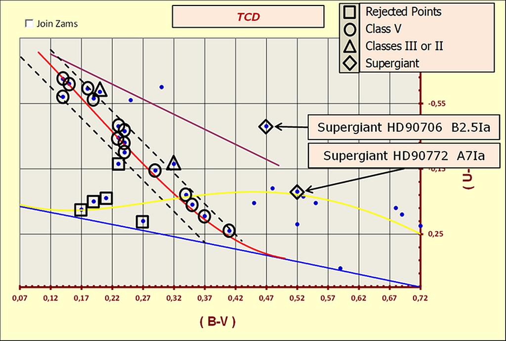
Figure - Capture of the class V early type stars at the blue-most envelope.

During the automatic acquisition, the code computes also the individual values for each early type star. Sometimes, however, the arrangement of the observed points on the TCD, is not as clear as in the case of IC2581. Several phenomena can scatter the observed data on the TCD. Among these phenomena, differential extinction often plays a prominent role, but it is not the only one. In absence of differential extinction, the code also tries to identify the evolving objects according to their position on the TCD. Later we will see how the code handles doubtful cases.

Perturbing phenomena on TCD.

Differential extinction occurs with greater intensity along the reddening lines relative to OB stars. It is the presence of randomly distributed matter within the cluster volume that causes the phenomenon of differential or non-uniform extinction. Although the differential extinction can be considered as the main element acting on the dispersion of the photometric sequences, it is not the only one and other processes can affect the dispersion, such as stellar evolution, stellar duplicity, stellar rotation, differences in chemical compositions, dispersion in ages, dispersion in distances, presence of non-members and last but not least, the limited precision of the de-reddened data Burki G. (1973) and (1975). [14] [15]

Cases of low differential extinction.

The distribution of the points for IC2581 in Figure 5 is obtained by plotting the original photometry of Lloyd Evans T. (1969). [16] The plot shows a clear case with a small amount of differential extinction. In such a situation it may be possible to discriminate automatically between luminosity classes. This can be done by considering the positions of the different stars on the two-colour diagram with respect to the paths of the luminosity calibrations II, Ib, Iab and Ia. The linear approximations used by the code for the luminosity classes used for this purpose are:

Evidently, there are several cases where the automatic selection between luminosity classes can be difficult or even impossible. In doubtful cases, the code asks for spectral data and luminosity class, especially for objects that appear to be evolving out of the main sequence. This is also the case for the uncertain position of the very bright yellow supergiant HD90772 of IC2581, see Figure 5. The code resolves the uncertainty by asking the user to enter a spectroscopic classification for HD90772. To obtain spectral data, the code freely connects to the WEBDA cluster site where such data can be retrieved. It is therefore clear that, in some situations, in addition to calculating each individual value for E(B-V), the code may attempt to recognize and manage evolving objects outside the main sequence. In all cases, the automatic discrimination is only possible if the differential extinction allows a correct interpretation of the luminosity classes on the TCD.

Cases of high differential extinction.

The methodology just seen cannot be applied in all cases. This is particularly true in the case of high differential extinction (very young clusters). In these cases, we must first determine the value of the differential extinction E(B-V) and then the value of the cluster <E(B-V)>. The effects of the differential extinction are important in very young clusters. Because of their young age, the material from which the stars were formed is still present. A detailed discussion about the differential extinction in open clusters, its effects and treatment, can be found in Burki G. (1975). [15] When there is a large amount of differential extinction, each individual E(B-V) is only obtained for stars with the value of the reddening free parameter Q = (U-B)-0.72(B-V) less than -0.38. Thus, following Golay (1974), [17] each individual E(B-V) value is obtained as:

Particularly reddened sky fields.

Sometimes, it can be difficult to obtain a correct value for <E(B-V)> using the sliding fit technique. This may be due to the presence of heavily obscured regions or particular scatter of data on TCD, as in the case of the default cluster Stock2. To overcome this obstacle, the user can always obtain spectroscopic data through the WEBDA database or the ADS literature search. With the spectroscopic data in hand, a call to the spectral de-reddening interface can solve the impasse. This utility, collecting associations between spectroscopic and photometric data, allows us to obtain the variable extinction diagram.

The main analysis menu.

The average colour excess <E(B-V)> is the only parameter required to access the main analysis menu (see Figure 6). From here, the user can perform various analyses related to the cluster under study. Everything happens under the control of this interface. For example, the user will not be able to access the data summary table without first determining the distance in the V₀ vs. (B-V)₀ plane and also in the V₀ vs. (U-B)₀ plane. An exception to this modus operandi is only possible for old clusters. Old clusters have no early type stars and therefore no fit on the V₀ vs. (U-B)₀ plane. In general, no analysis can be performed without first determining the distance. After obtaining the distance modulus for the cluster under study, the code offers several procedures, such as:

• A table containing the intrinsic individual data for all programmed stars.

• The colour-absolute magnitude diagram.

• The semi-empirical tracks comparison interface.

• The Log (T_eff) vs. Log (L/L_s) interface.

• The Log (T_eff) vs. M_Bol interface.

• The metallicity interface.

• The final data interface.

• The internal WEBDA data interface.

Figure - A view of the main analysis menu.

Determining the true distance modulus <V_o-M_V>.

As previously said, the size of an open star cluster is small if compared to its distance from us. For this reason, we can consider all members of the cluster at the same distance from us. If this is a reasonable idea, the V apparent magnitude of the cluster members differs from absolute magnitudes M_V by the same amount V-M_V and we can refer this quantity as distance modulus. By arranging, on a diagram, the apparent magnitudes of the stars with respect to their spectral types or colour indices, the resulting array is essentially a spectrum or colour index vs. an absolute magnitude calibration, except for the distance modulus difference. The method used by the code to determine the distance of a galactic cluster, the is the Zero Age Main Sequence (Zams) fitting. To achieve this result, the code relies on the Schmidt-Kaler (1982) absolute magnitude empirical calibration. [4] The prerogative of this calibration is to relate the de-reddened (B-V)₀ colour index to the absolute magnitude M_V. Therefore, the distance modulus of any cluster can be obtained by matching the comparable parts between our calibration and the cluster array on a (B-V)₀, vs. V₀ diagram. This gives the difference between the apparent and the absolute magnitudes. The code performs this comparison in two different ways: automatically or graphically. In both cases, the empirical Zams is shifted downwards until the best fit with the lower envelope of the cluster array is obtained. As for the TCD interface, the Zams is obtained with a 6^th order interpolating polynomial. According to the general polynomial expression, the zero-age main sequence locus is represented by the following equation (16):

Using equation (16), the code calculates each individual distance modulus. It then averages all the individuals (V₀-M_V), to obtain the true average distance modulus <V₀-M_V> of the cluster. The mathematical best-fit procedure works in a fully automatic mode. On the contrary, when using the manual procedure and remembering that the Zams is defined as the low luminosity locus Balona L.A. (1984), the user must move the Zams down, step by step, until the best fit with the lower luminosity envelope of the cluster array is obtained. [18]

An example with IC 2581 <Vo-M_V> determination.

Figure 7 shows an example with IC 2581 photometric data on a (B-V)₀, vs. V₀ plane. The cluster shows a well-defined main sequence in the range -0.26≤ (B-V)₀ ≤0.17. The blue turn-off point is visible around (B-V)₀ = -0.27. The scatter of the observed points for IC 2581 with respect to V₀ is very small. The value of the selected turn-off point is used by the code to calculate the cluster age with the Maeder A., Meynet G., and Mermilliod C. calibration (1993). [19] Figure 8 shows the mathematical fit. The true distance modulus obtained is: 12.34 ± 0.1 magnitudes. Following W. Becker (1963) and (1966), we must repeat the same fitting procedure using the (U-B)₀ vs. V₀ plane, as shown in Figures 9, 10 and then average the values. [20] [21]

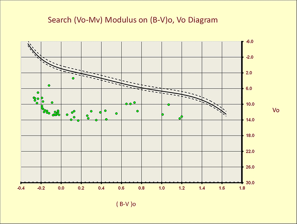
Figure - IC2581 <V₀-Mv> determination. The starting situation on the (B-V)₀ vs. Vo plane.

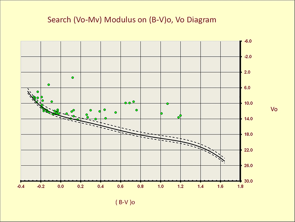
Figure - The IC2581 array fitted for <Vo-Mv> = 12.34 ± 0.1 on the (B-V)₀ plane.

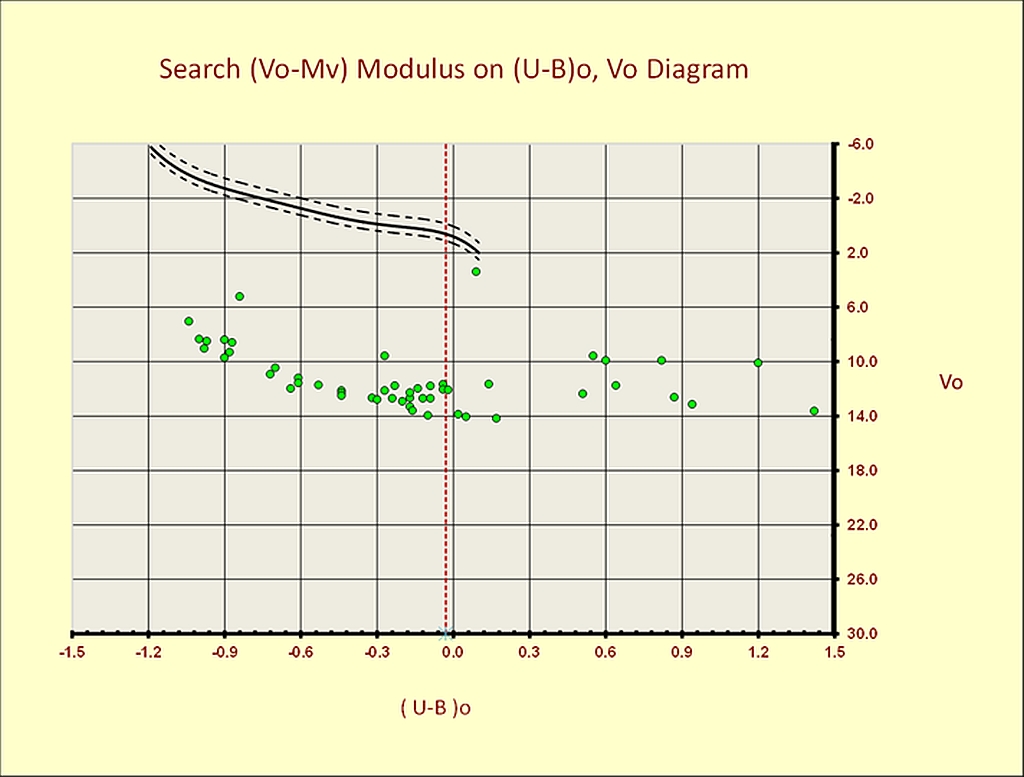
Figure - IC2581 <V₀ -Mv> determination. The starting situation on the (U-B)₀ plane.

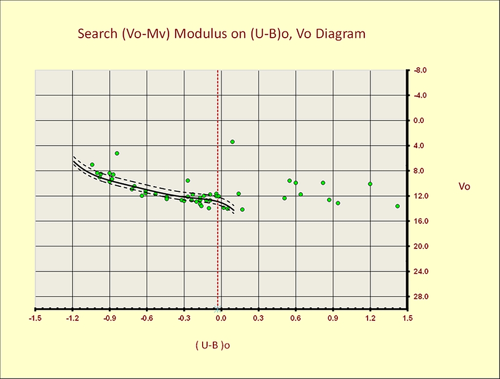
Figure - The IC2581 array fitted for <V₀ -Mv> = 12.27 ± 0.38 on the (U-B)₀ plane.

Averaging the two distances we have: <V₀-M_V> = 12.36±0.27. Using the variable extinction method Turner D.G. (1978) obtained 12.29±0.12. [22] Despite different methods the agreement between the results seems to be good.

Selection of cluster members.

The selection for cluster membership is not straightforward and can be made through various criteria, namely photometric, kinematic, statistical and spectroscopic. The code does not provide for membership analysis. This complex analysis is left to a preliminary study, which should eliminate spurious data before the photometric analysis. The presence of spurious data increases the scatter and worsens the results. Nevertheless, on the clean data, the code can apply the group membership criterion as proposed by Walker G.A.H. (1965). [23] This implies that a member should have a distance modulus no more than 0.5 mag. from the mean modulus and the duplicity should not brighten a star more than 0.75 mag. from the mean modulus. Walker’s criterion is only reliable for main sequence stars.

The colour vs. absolute magnitude diagram.

If we know the distance, we also know the absolute magnitudes, so a colour vs. absolute magnitude diagram can be plotted. Figure 11 shows this for IC2581. We can see that this cluster is young and formed by stars in the early spectral classes, with surface temperatures ranging from 8000° K to 27000° K. Even the photometric radii of certain stars are considerable. The values computed by the code, using the calibration of Wesselink A.J. (1969), are in the range R/R_S = 2.2 to R/R_S = 258, where R_S is the Solar radius taken as unitary. [24]

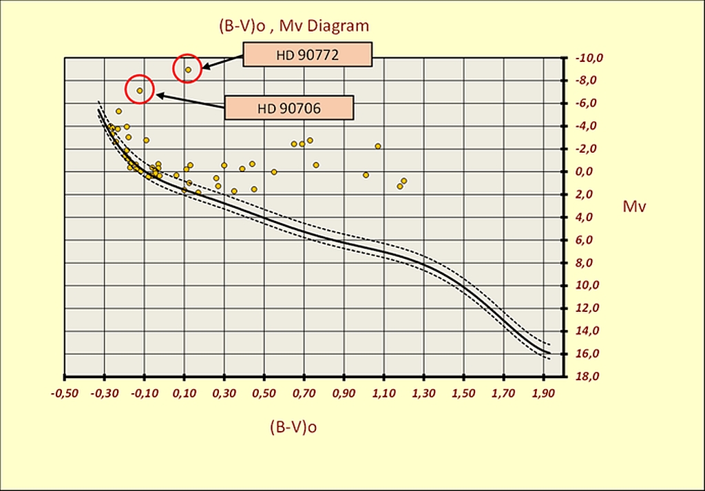
Figure - The IC2581 Colour-absolute magnitude diagram.

The higher computed values are those for HD90772 and HD90706 - two bright supergiants. There are many studies in the literature about IC2581 its supergiants and the value of R in the cluster region. Turner D.G. studied this cluster extensively in (1978). [22] From spectroscopic and photometric studies, the author obtained the following values for the two supergiants:

• HD90772 spectral type A7Ia0 with M_V -8.8

• HD90706 spectral type B2.5Ia with M_V -7.2

respectively. If we compare the automatic code results with the Turner D.G. data, we can observe a substantial agreement. (See Table 1 and Figure12).

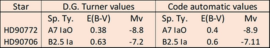
Table - Comparison D.G. Turner vs. Code.

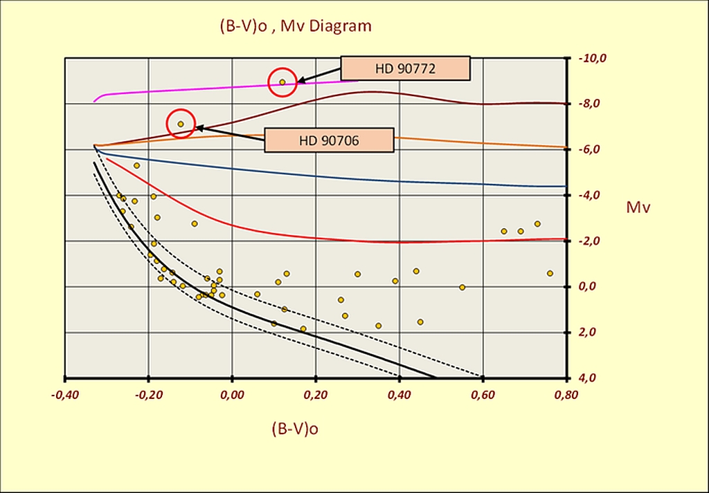
Figure - IC2581 identification of HD90772 and HD90706 along their luminosity classes Ia0 and Ia respectively.

Although the results are based on different distance determination methods, they appear to be very similar. It may still be interesting to evaluate how the code identifies the spectral type and luminosity class of HD90706. From Turner’s study we know that the spectral class of HD90706 is: B2.5Ia. The Schmidt-Kaler 1982 calibration assigns the following un-reddened values to spectral classes B2Ia and B3Ia:

• B2Ia (B-V)₀ = -0.16 and (U-B)₀ = -0.96

• B3Ia (B-V)₀ = -0.12 and (U-B)₀ = -0.85

respectively. The results provided by the code for HD90706 are: (B-V)₀ = -0.127 and (U-B)₀ = -0.844. This means that HD90706 is identified photometrically as an intermediate star between the B2Ia and B3Ia classes. It is also worth noting the ratio between the radii of the two most luminous stars, that turns out to be (HD90772/ HD90706) = 3.67. The ratio between the radii of these two supergiants must be considered according to the effective temperature of the two stars, calculated by the code using the Flower calibration (1966) as 8298° K for HD 90772 and 15353° K for HD90706. [25] Obviously, the colder body needs a larger radiating surface compared to the warmer body to reach its M_V = - 8.9. This situation is well explained by the Stefan-Boltzmann law (17).

Where, L is the luminosity in Watts, R is the radius in metres, T is the surface temperature in Kelvin and is Stefan-Boltzmann constant

The HR theoretical diagrams log (L/L_s) vs. log (T_eff) and log (T_eff) vs. M_Bol.

In order to convert the intrinsic colours into effective temperatures, the code uses data from P. Flower (1975), (1977) and (1996). [25] [26] [27] The polynomial equation used to obtain the effective temperature (T_eff) from the intrinsic colours is similar to the previous ones except for the polynomial degree, here a 7^th degree is used. The computation of the quantity Log (L/L_S) for each member is obtained by equation (18).

Where L_S is the solar luminosity taken as unitary, BC is the bolometric correction and DM is the true distance modulus <V₀-M_V>. The transition from the CM colour-magnitude diagram to the HR diagram requires two conversions: the colour index must be converted to effective temperature and the absolute magnitude must be converted to bolometric magnitude. In both cases, the method used by the code to perform the calculations is always the same. The relationship between absolute magnitude and bolometric magnitude is:

The bolometric corrections are determined by the code using the Log (T_eff) and BC tables of H.L. Johnson (1966) and P. Flower (1996). [28] [27] Within the preliminary theoretical interface Figure 13, some comparisons can be made with a series of stellar models from V. Castellani, A. Cheffi and O. Straniero stellar models (1993), in the range from 30 Myr to 10 Gyr.

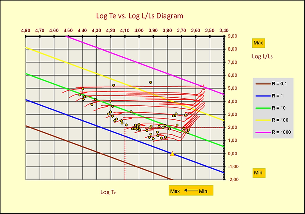
Figure - IC2581 on the preliminary theoretical interface.

The yellow-red triangle in Figure 13 shows the solar position.

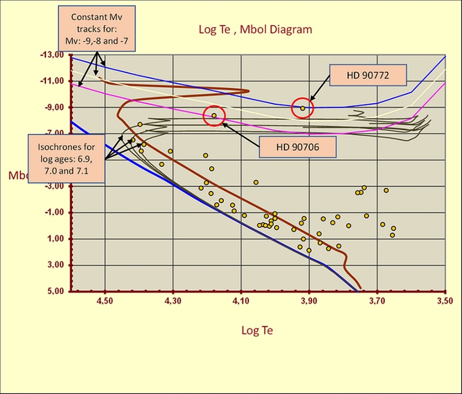
Figure - IC2581 on the most complete theoretical interface made available by the code.

A more advanced analysis is possible using the T_eff, vs. M_bol diagram. Figure 14 shows this successive most complete theoretical interface provided by the code. Superimposing the evolutionary tracks on the IC 2581 array in this interface, we see that the majority of the members of this cluster are made up of stars between 2 to 15 solar masses. Only HD 90772 and HD 90706 have higher values - between 20 and 30 solar masses - as might be expected given the absolute high magnitudes of these stars. We can then overlay a series of isochrones on the cluster sequence for evaluations. The same interface also gives the cluster age from the blue turn-off value. This value is obtained using the calibration of A. Maeder, G. Meynet, and C. Mermilliod. [29] Besides, always in this interface, the user can compare the clusters under study, according to the following utilities:

• Constant magnitudes M_V tracks in a range between -5Mv to -9Mv.

• Geneva models tracks in a range between 1 to 120 solar masses and metallicities for Z=0.02 and Z= 0.001 Schaller & co-workers, (1992). [30]

• Isochrones for metallicities Z=0.02, Z=0.008 and Z=0.004 and ages from 6.6 to 10.30 log(ages). Padua group Bertelli & co-workers, (1994). [31]

In addition, and always from this interface, the user can obtain the cluster present day mass function (PDMF). At the end of each analysis, the results are summarised in the final tab interface. See table 2.

The final data interface.

Table 2 shows a view on the final data interface for the analysis of the cluster IC2581.

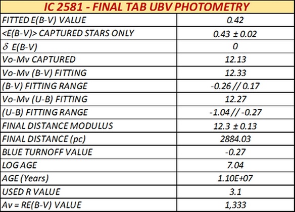
Table - View of the final results for IC2581

Variable phenomena inside Open Clusters.

Stellar variability within or around open clusters, could reveal interesting possibilities. Within clusters, we may encounter different types of variable phenomena affecting the population I stars. The user can identify possible variable objects using either the Log (T_eff) vs. M_bol or the HRD Regions & Instability Strips interfaces (see Figures 15 and 16). Figure 15 illustrates the supergiant HD90772 as an extremely interesting object located next to the border between the area of the A Supergiants and Hypergiants. Due to its position on the HRD, HD90722 alias V399 Carinae is a variable star, catalogued from the recent Hipparcos 2011 photometry as:  Cygni variable with a V amplitude range between +4.63 and +4.72. Another interesting cluster on this interface is NGC4755 with its red supergiant CPD-59°.4547. Again, this star occupies a very interesting position on the diagram, as it is lies at the upper boundary between the M Supergiants and Hypergiants area (Figure 16). Also, CPD-59°.4547 alias DU Crucis due to its position on the HRD, turns out to be a variable star catalogued as: Lc type slow irregular variable. The HRD region interface can help us to identify stars belonging to the HR instability strips or regions, including variable objects such as  cephei, SPB (Slowly pulsating B stars),  Scuti and so on. On the other hand, within very young clusters, the user may encounter variability associated to very massive objects, such as LBVs, Wolf-Rayet, and OB massive stars. Intermediate age clusters may host variability associated to yellow supergiants, or population I cepheids. Sometimes, young and intermediate age clusters can also contain some evolved objects, such as red supergiants, with their variable phenomena.

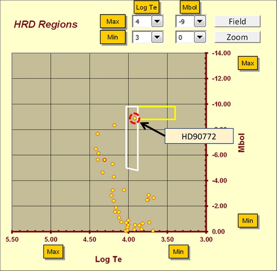
Figure 15 - HD90772 at the border between the A supergiant area and Hypergiant area.

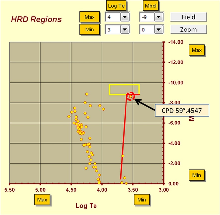
Figure 16 - CPD -59°.4547 at the upper border between the Red giant area and the Hypergiant area.

Finally, in many young clusters, there is also the possibility to study T-Tauri stars; another class of eruptive variables related to the pre-main sequence phase or newly formed stars. T-Tauri variability is mostly due to flaring phenomena. In addition, the study of binary stars in clusters can yield other important results. In the case of binaries, we know that by combining spectroscopic and photometric data together, we can also determine the distance.

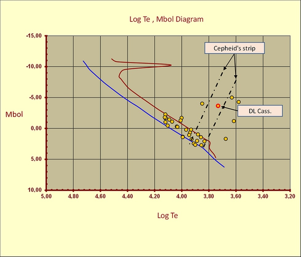
Figure 17 - DL Cass. found within the Cepheid's instability strip.

Moreover, some categories of variable stars - if included in clusters - allow us to compare the resulting Zams fitting distance. For instance, we can compare distances using the Cepheid Period-Luminosity relations. Figure 17 shows how the code identifies the Cepheid DL Cassiopeia member of the cluster NGC 129 within the Cepheid’s instability strip. However, the Cepheids are not the only type of stars that can be used. Contact binaries can also be used. A good example of these comparisons for contact binaries can be seen in Mochejska B.J. & Kaluzny J. (1999). In their work on the intermediate age open cluster NGC 7789, the authors found 35 W Ursae Majoris systems in the cluster field. To assess the cluster membership of contact binaries, the authors applied the absolute magnitude calibration of Rucinski & Duerbeck (1997), see the following equation (20). [32] [33]

Where P is the period of the contact binary in days. As a result of the calculations using equation [20], at least 5 systems seem to be cluster members with computed distances within ± 0.2 compared to the distance of the suspected parent cluster. Others similar comparisons can be made, for instance, using  scuti stars whenever possible.

The BVIc photometry.

For BVIc photometry, the behaviour of the code is quite different from that for UBV photometry. For this type of photometry, the code does not provide automatic fitting procedures, and in general there are few automatic procedures. The user involvement is therefore essential. The main obstacle we encounter here is that with two temperature sensitive indices the determination of reddening is practically impossible because the slope of the reddening line coincides with the array of photometric data. Therefore, there are basically two ways to proceed with this system:

• The first option is: to find the value of the reddening parameter <E(B-V)>, for the cluster under study, consulting the technical literature or databases such as WEBDA.

• The second option - widely applied by professionals - involves the simultaneous determination of reddening and distance by comparing the photometry with a series of isochrones from stellar models on (B-V) vs. V or (V-I) vs. V diagrams.

Figures 18, 19, 20, and 21 show, step by step, the code simultaneous determination of reddening and distance for the cluster NGC 2516 as follows:

• Reddening <E(B-V)> = 0.101

• Distance modulus < (V₀ - M_V) = 8.16±0.33

• Log Age = 8.1 about 125.9 Myr.

Table 3, instead, shows the final data table. Adopting this methodology, the code is able to provide help because it contains an internal version of the WEBDA database, as well as an internal database for the isochrones of the Padua group with the following metallicities: Z=0.02, Z=0.008 and Z=0.001 Bertelli G. (1994). [31] Obviously, comparisons between observational data and theoretical isochrones can be made on both planes (B-V) vs. V and (V-I) vs. V. However, in order to use this method profitably, the presence of evolving stars outside the main sequence is required.

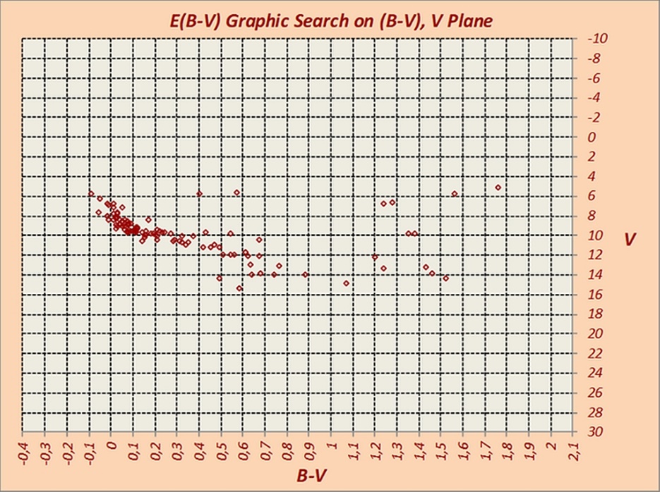
Figure 18 - The cluster NGC2516 on the (B-V) vs. V diagram.

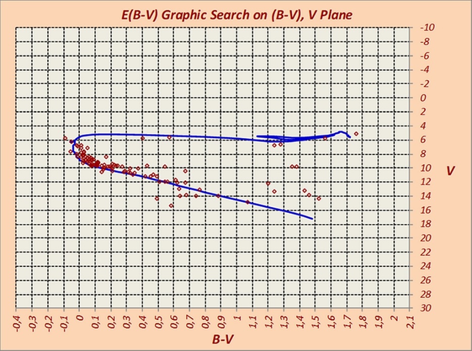
Figure 19 - The rough isochrones fitting based on WEBDA mean data.

The presence of evolved stars is important as all isochrones fit the entire main sequence very well. So, the presence of stars evolved outside the main sequence allows a better determination of the fit in terms of reddening, distance, and age. In practice, using isochrones, we should always look for the best fit between the turn-off point and the clump of the red giants, in both diagrams (B-V) vs. V and (V-I) vs. V.

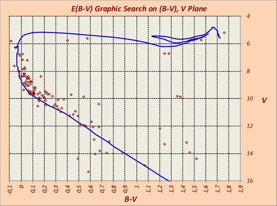
Figure 20 - An enlargement of the WEBDA rough fit.

Figure 21 - The NGC2516 fine final fit.

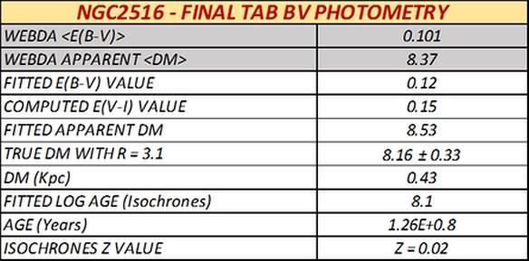
Table - Final results for NGC251 BVIc photometry.

Conclusions.

As data interpretation may not always be so easy, the use of this code should provide the possibility to carry out a complete study. The code can be obtained - free of charge - from the author - via the following e-mail address: valter.arno51@gmail.com

Acknowledgements

The development of this application was made possible thanks to Microsoft’s publications on VBA (Visual Basic for Application). This programming language allows us to manipulate Excel beyond its standard capabilities. Other essential data for this study, such as photometric values and technical literature, were obtained thanks to the WEBDA and NASA-ADS websites.

Valter Arnò e-mail address: valter.arno51@gmail.com

References

1. Johnson, H. L. et Al. – 1953 Ap. J. 117, 313
2. Cousins, A.W. J. – 1978 MNASSA 37, 62
3. Heintze J.R.W – 1973 IAUS 54, 231
4. Schmidt-Kaler Th. – 1982 Landolt Bornstein Group IV, Vol. 2 Stars and Star Clusters
5. Turner D.G. – 1989 A.J. 98, 2300
6. Turner D.G. – 1994 Rev. Mex. de Astronomia y Astrofisica 29, 163
7. Dean W.W., Warren P.R., Cousins A.W.J. – 1978 MNRAS 183, 569
8. Pollacco D.L. – 1989 PhD thesis St. Andrews
9. Pollacco et Al. – 1992 MNRAS 254, 228
10. Schmidt-Kaler Th. – 1961 Z. Astrophys. 53, 1
11. Fernie J.D. – 1963 A.J. 68, 780
12. Turner D.G. – 1976 A.J. 81, 97
13. Johnson, H. L. – 1968 Nebulae and Interstellar Matter Chicago U. P.
14. Burki, G. et Al. – 1973 A.& A. 25, 78
15. Burki, G. – 1975 A.& A. 43, 37
16. Lloyd Evans T. – 1969 MNRAS 146, 101
17. Golay, M. 1974 -Introduction to Astronomical Photometry D. Reidel Publishing Company.
18. Balona, L. A. et Al. – 1984 MNRAS 211, 375
19. Maeder, A. et Al. – 1993 A. & AS. 98, 477
20. Becker, W. et Al. – 1963 Z.A. 57, 117
21. Becker, W. et Al. – 1966 Basic Astronomical Data Ed. K. AA Strand Chicago U. P.
22. Turner D.G. – 1978 A.J. 83, 1081
23. Walker G.A.H. – 1965 Ap. J. 141, 660.
24. Wesselink A.J. – 1969 MNRAS 144, 297
25. Flower P. J. – 1975 A&A 41, 391
26. Flower P. J. – 1977 A&A 54, 31
27. Flower P. J. – 1996 Ap.J. 469, 355
28. Johnson, H. L. – 1966 ARA & A. 4, 193
29. Castellani, V. – 1990 Ap.J.S. 463, 494
30. Shaller G. et Al. – 1992 A&AS 96, 269
31. Bertelli G. et Al. – 1994 A. & AS. 106, 275
32. Mochejska B. J. et Al. – 1999 AcA 49, 351
33. Rucinski S. M. et Al. – 1997 PASP 109, 1340
34. Straižys V. – 1992 Multicolor Stellar Photometry Pachart Publishing House – Tucson